Experiment

---

1 Getting started

To copy the code, click the button in the upper right corner of the code-chunks.

1.1 clean up

rm(list = ls())
gc()

1.2 custom functions

We defined a number custom functions, at Download custom_functions.R.

source("./custom_functions.R")

1.3 necessary packages

• tidyverse: data wrangling
• igraph: generate and visualize graphs
• parallel: parallel computing to speed up simulation
• foreach: looping in parallel
• doParallel: parallel backend for foreach
• ggplot2: data visualization
• ggh4x: hacks for ggplot2
• ggpubr: make visualizations publication-ready

packages = c("tidyverse", "igraph", "ggplot2", "parallel", "doParallel", "foreach", "ggh4x", "ggpubr",
    "plotly", "RColorBrewer", "grid", "gridExtra", "patchwork", "ggplotify", "ggraph", "gganimate", "RColorBrewer",
    "ggtext", "magick", "jsonlite")

invisible(fpackage.check(packages))
rm(packages)

---

2 Experimental conditions

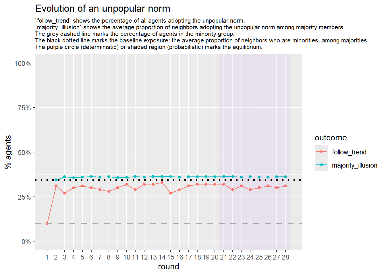
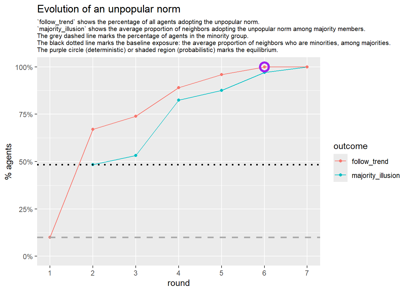
2.1 1. heavy-tailed network with central minorities

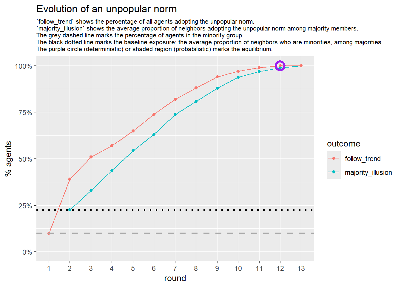
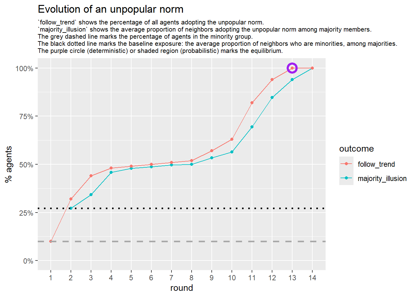
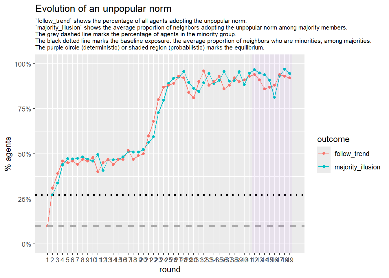
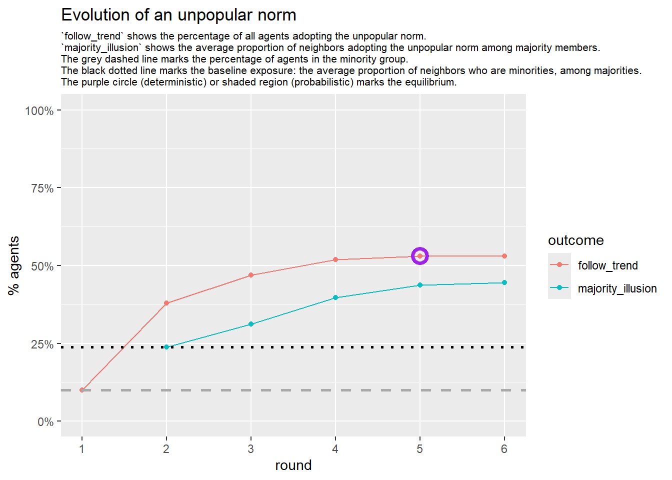
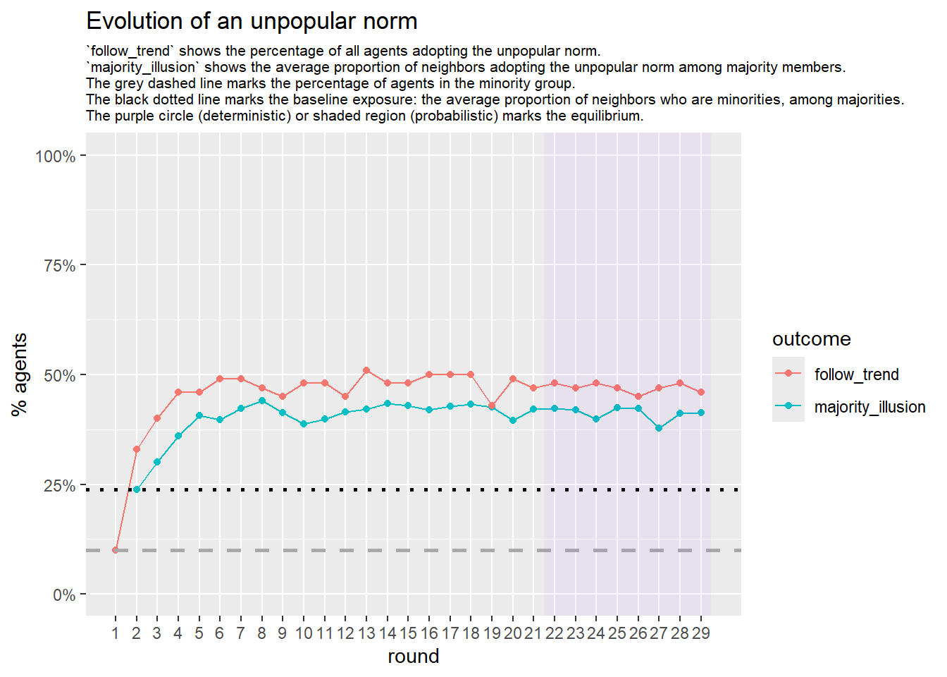
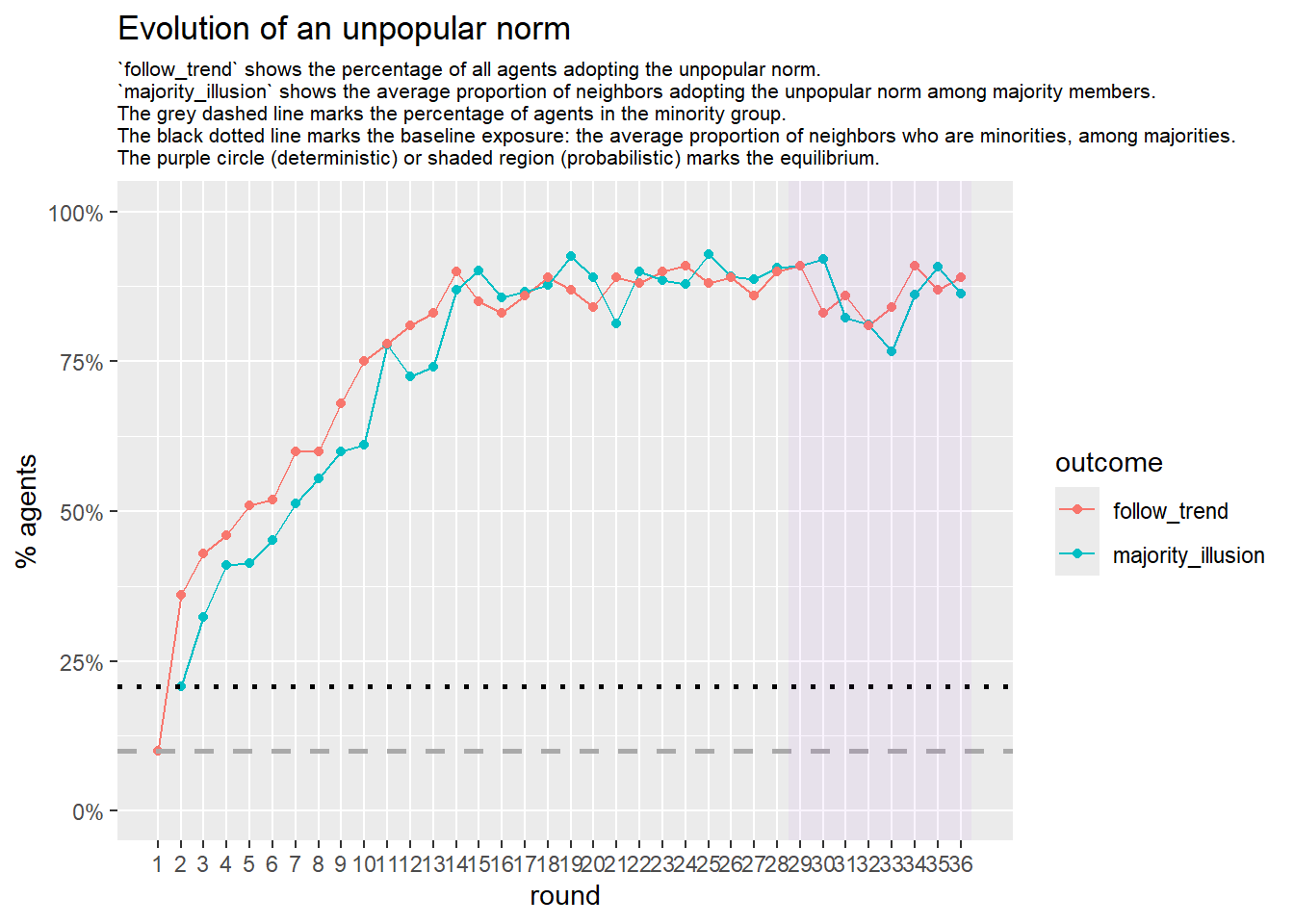
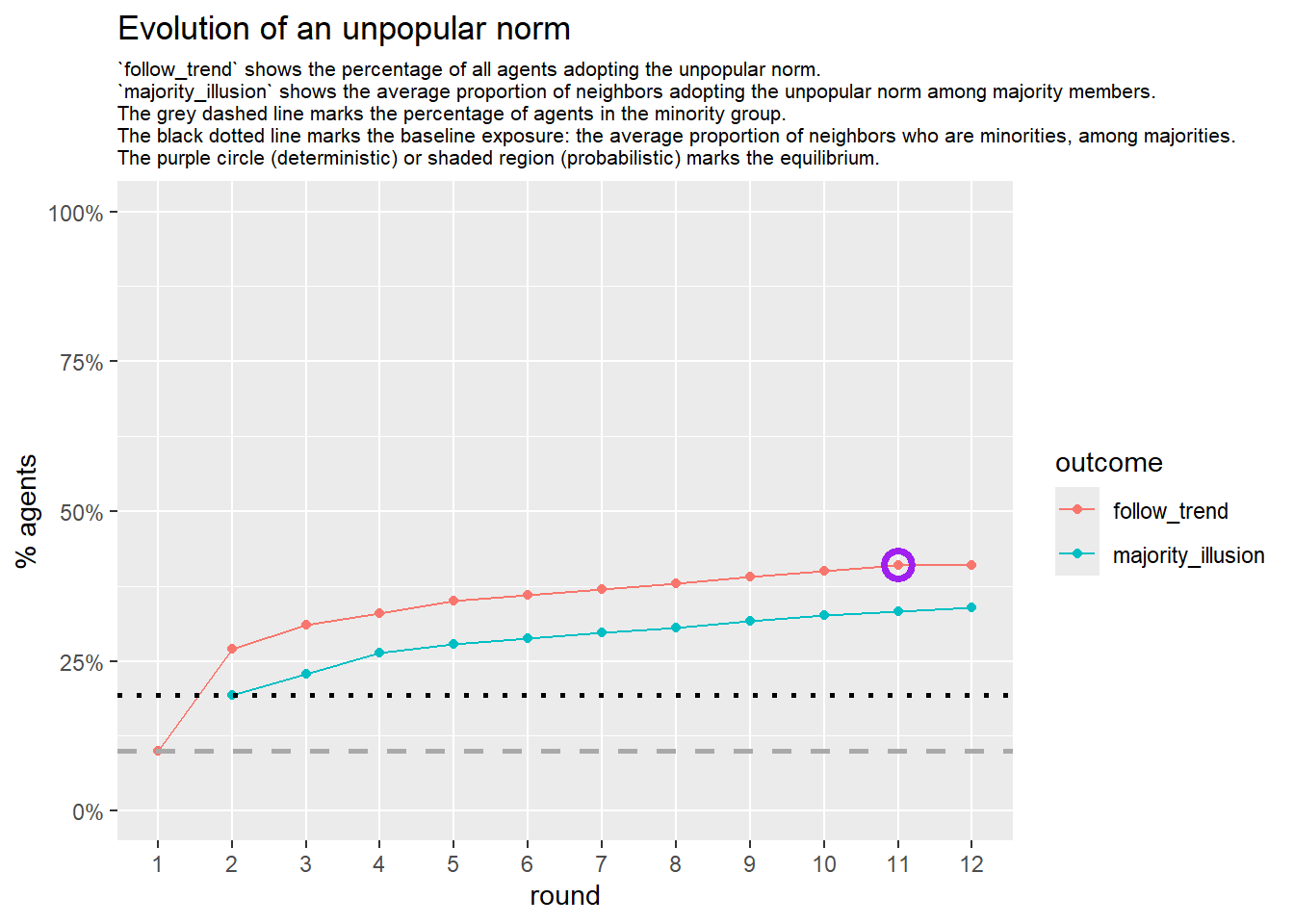
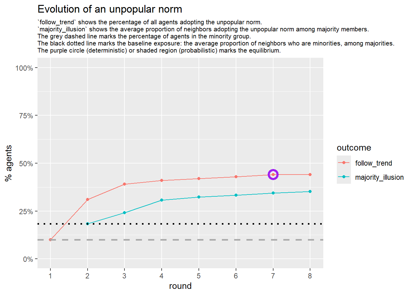
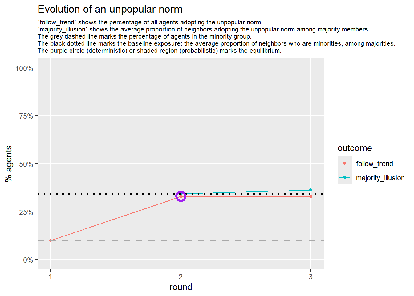
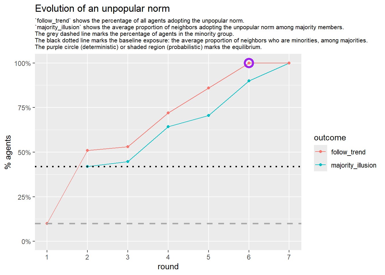
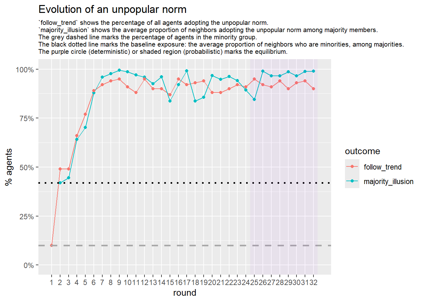
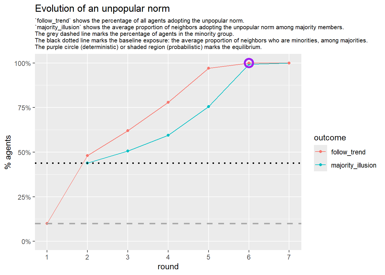
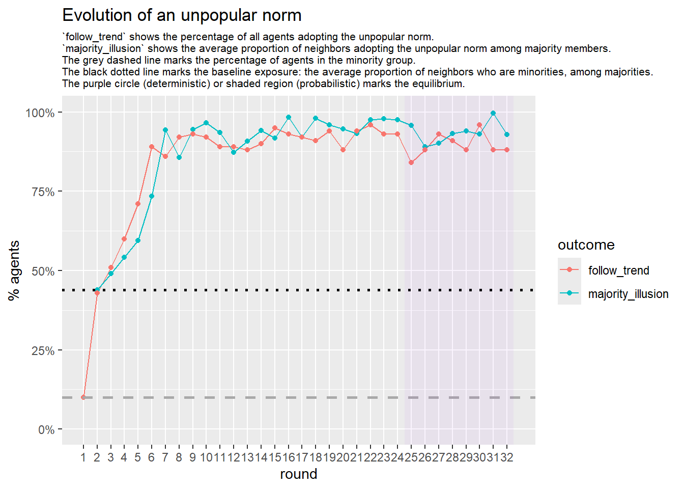
Let’s take a likely-case for an unpopular norm, generate multiple networks of this target, and simulate the emergence of the norm following a deterministic and probabilistic choice model:

# pick one configuration that likely leads to an unpopular norm, and explore multiple 'seeds':
run_one_seed <- function(
  i,
  base_seed = 1253281,
  params = list(s = 15, e = 10, w = 40, z = 50, lambda1 = 5, lambda2 = 1.8),
  
  # tweak network
  k_min = 2, 
  k_max = 20,
  alpha = 2.4,
  rho = 0.4,
  r = -0.1,
  
  # retrieve network
  return_network = FALSE
  
) {
  # derived seed for this run
  seed_i <- base_seed + i
  set.seed(seed_i)

  # --- network creation ---
  degseq <- fdegseq(
    n      = 100,
    alpha  = alpha,
    k_min  = k_min,
    k_max  = k_max,
    dist   = "log-normal", #use log-normal 
    seed   = seed_i
  )

  network <- sample_degseq(degseq, method = "vl")
  
  V(network)$role <- sample(
    c(rep("trendsetter", 10), rep("conformist", 90))
  )
  

  rewired_network <- frewire_r(network, r, verbose = FALSE, max_iter = 1e5)
  final_network   <- fswap_rho(rewired_network, rho, verbose = FALSE, max_iter = 1e4)
  
  # --- stats ---
  stats <- list(
    run           = i,
    seed          = seed_i,
    num_nodes     = vcount(final_network),
    num_edges     = ecount(final_network),
    avg_degree    = mean(degree(final_network)),
    sd_degree     = sd(degree(final_network)),
    net_density   = edge_density(final_network),
    net_diameter  = diameter(final_network, directed = FALSE, unconnected = TRUE),
    avg_path_len  = average.path.length(final_network, directed = FALSE),
    clust_coeff   = transitivity(final_network, type = "global"),
    assort_deg    = assortativity_degree(final_network),
    deg_trait_cor = fdegtraitcor(final_network)$cor,
    components    = components(final_network)$no
  )
  
  fplot_graph(final_network, layout = layout_with_fr(final_network)) 
  
  
  # --- initial actions ---
  V(final_network)$action <- ifelse(V(final_network)$role == "trendsetter", 1, 0)
  
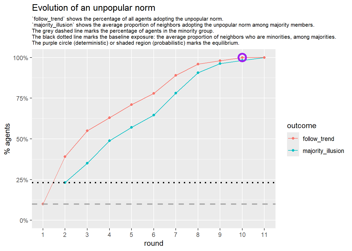
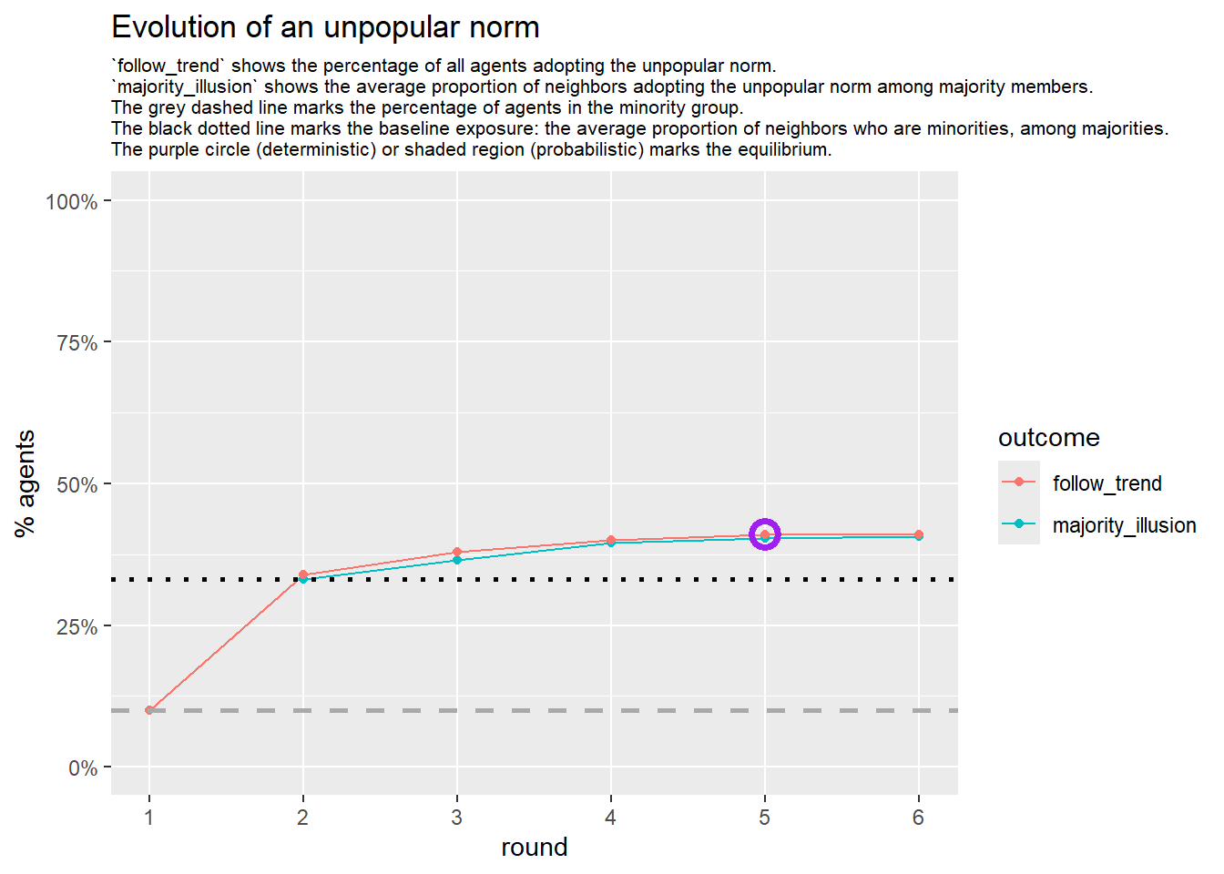
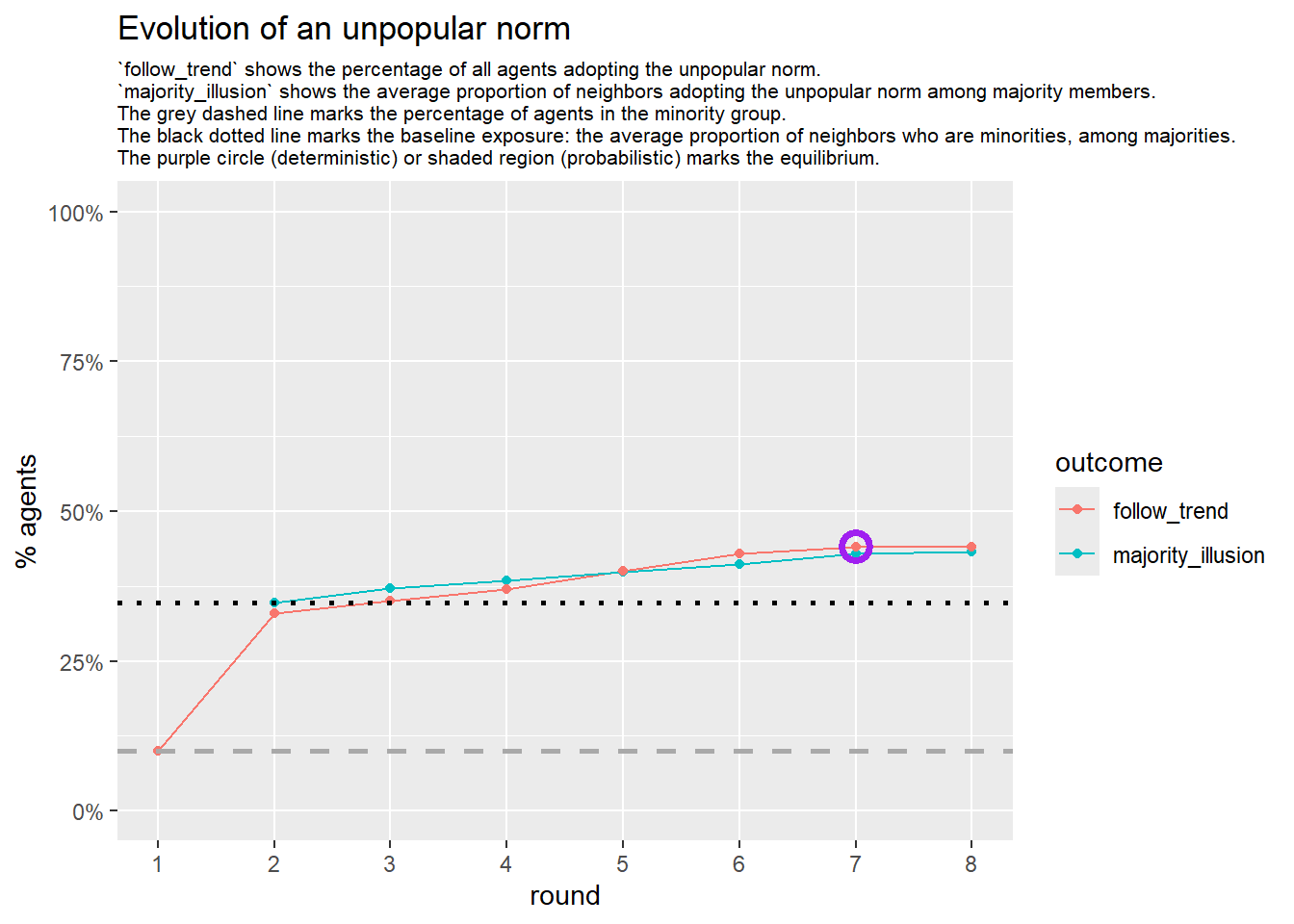
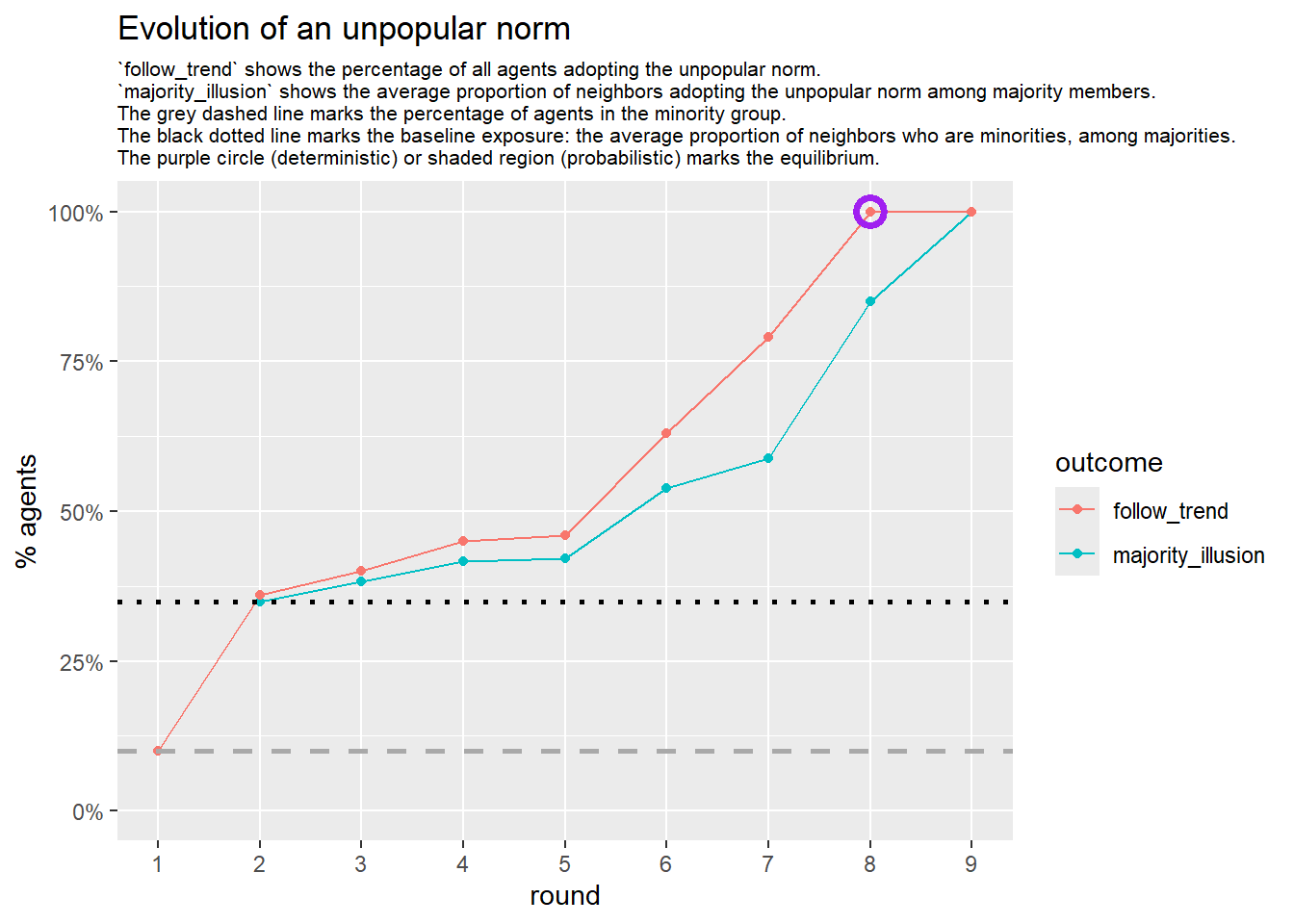
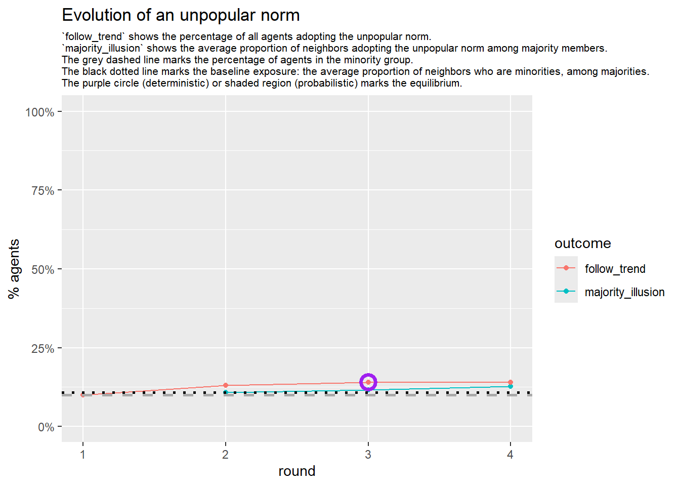
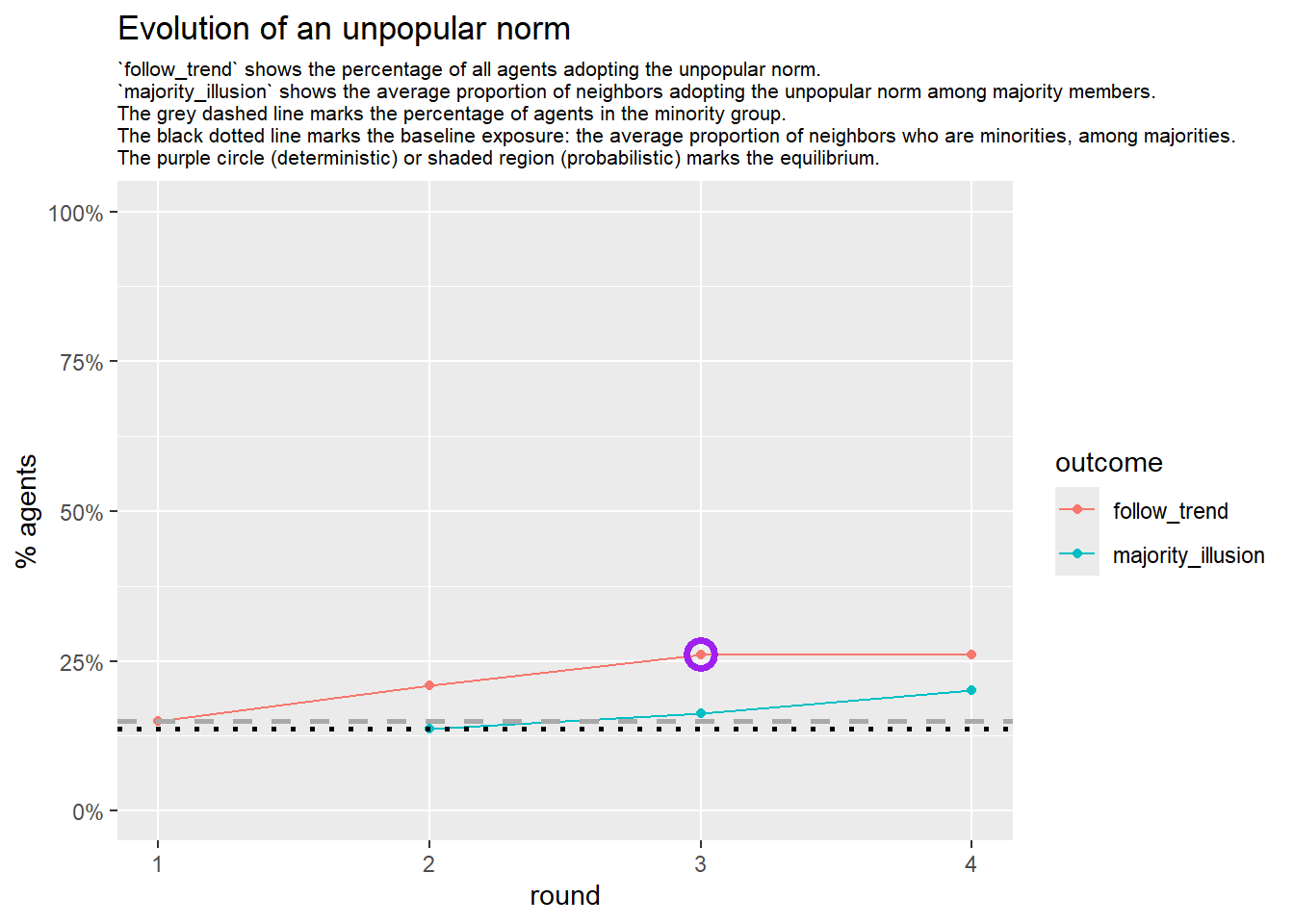
  # --- deterministic simulation ---
  sim_det <- fabm(
    network      = final_network,
    params       = params,
    max_rounds   = 50,
    mi_threshold = 0.49,
    choice_rule  = "deterministic",
    plot         = TRUE,
    histories    = TRUE
  )
  
  # generate the gif for the current network
  gif_filename <- paste0("./figures/animation_network_", seed_i, ".gif")
  gif_path <- fnetworkgif(final_network, sim_det$decision_history, rounds = sim_det$equilibrium$round, output_dir = "./figures")
  # rename the gif to match the naming pattern
  file.rename(gif_path, gif_filename)

  if (!is.null(sim_det$plot)) {
    print(sim_det$plot)
  }
  
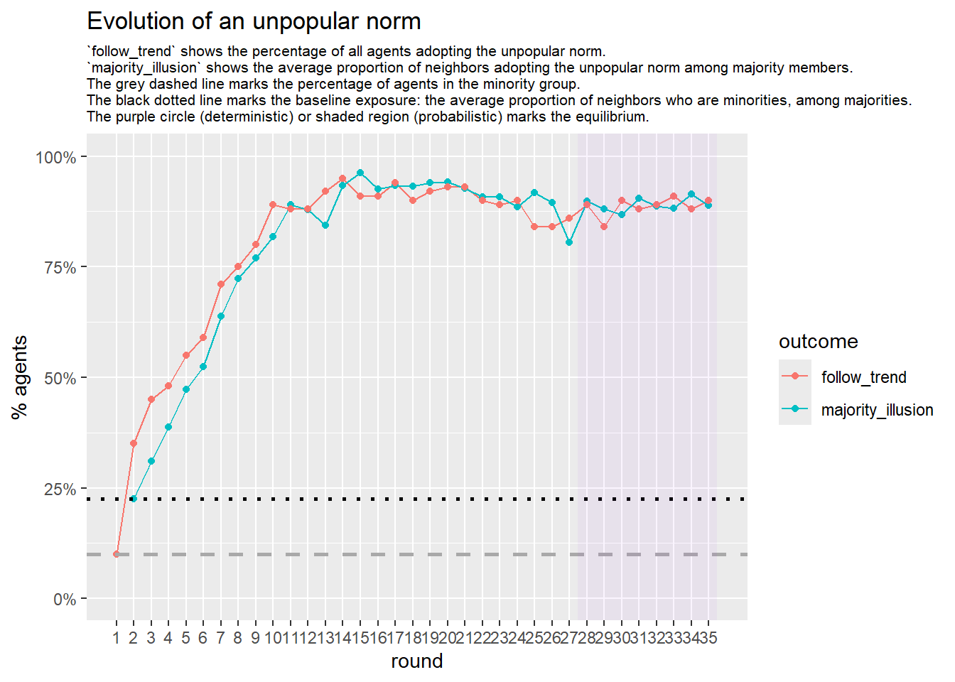
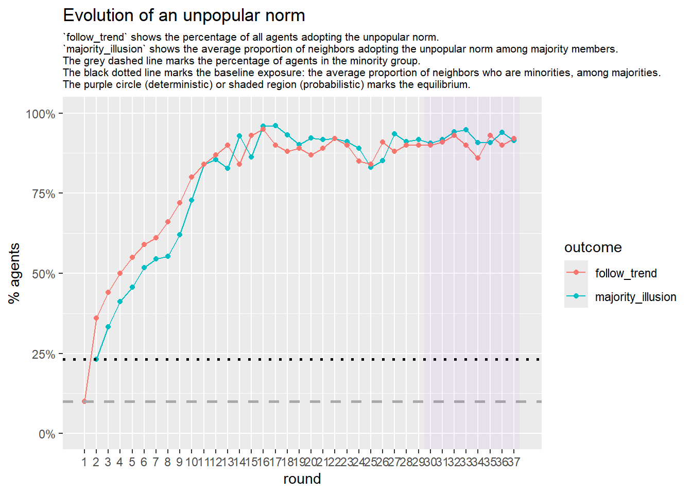
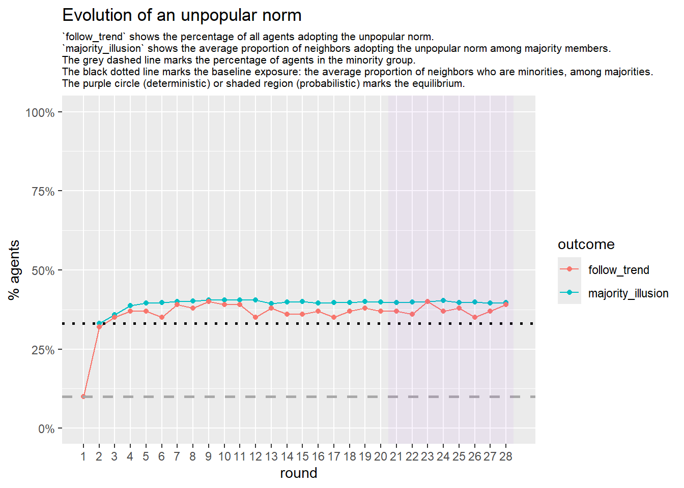
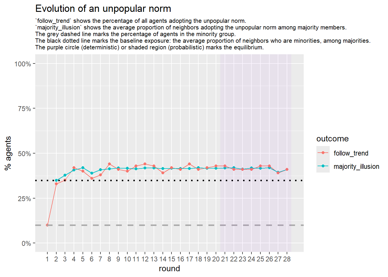
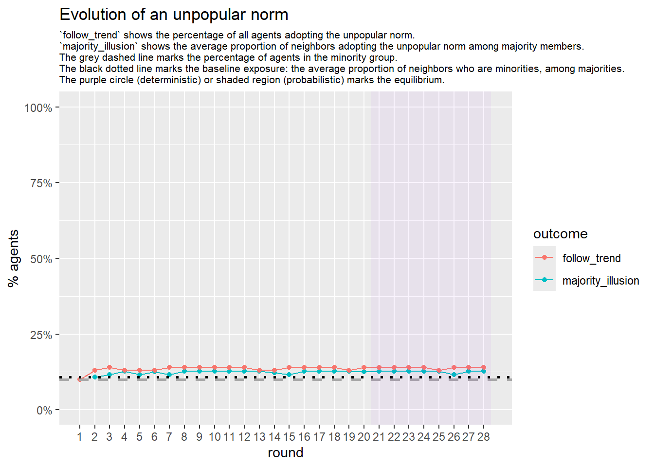
  # --- probabilistic simulation ---
  sim_prob <- fabm(
    network                = final_network,
    params                 = params,
    max_rounds             = 100,
    mi_threshold           = 0.49,
    choice_rule            = "probabilistic",
    stable_window          = 8,   # the length of the window of adoption values
    required_stable_rounds = 20, # number of windows needed to declare equilibrium
    plot                   = TRUE
  )
  if (!is.null(sim_prob$plot)) {
    print(sim_prob$plot)
  }
  
   result <- list(
    segregation_det  = sim_det$equilibrium$segregation,
    segregation_prob = sim_prob$equilibrium$segregation,
    stats            = stats
  )
  
  if (return_network) {
    result$network <- final_network
  }
  
  result
}

test <- run_one_seed(1, k_min = 2, k_max = 20, alpha = 2.4, rho = 0.4, r = -0.1, return_network = TRUE)

base = 1253281
seed = base + 1

knitr::include_graphics(paste0("./figures/animation_network_", seed, ".gif"))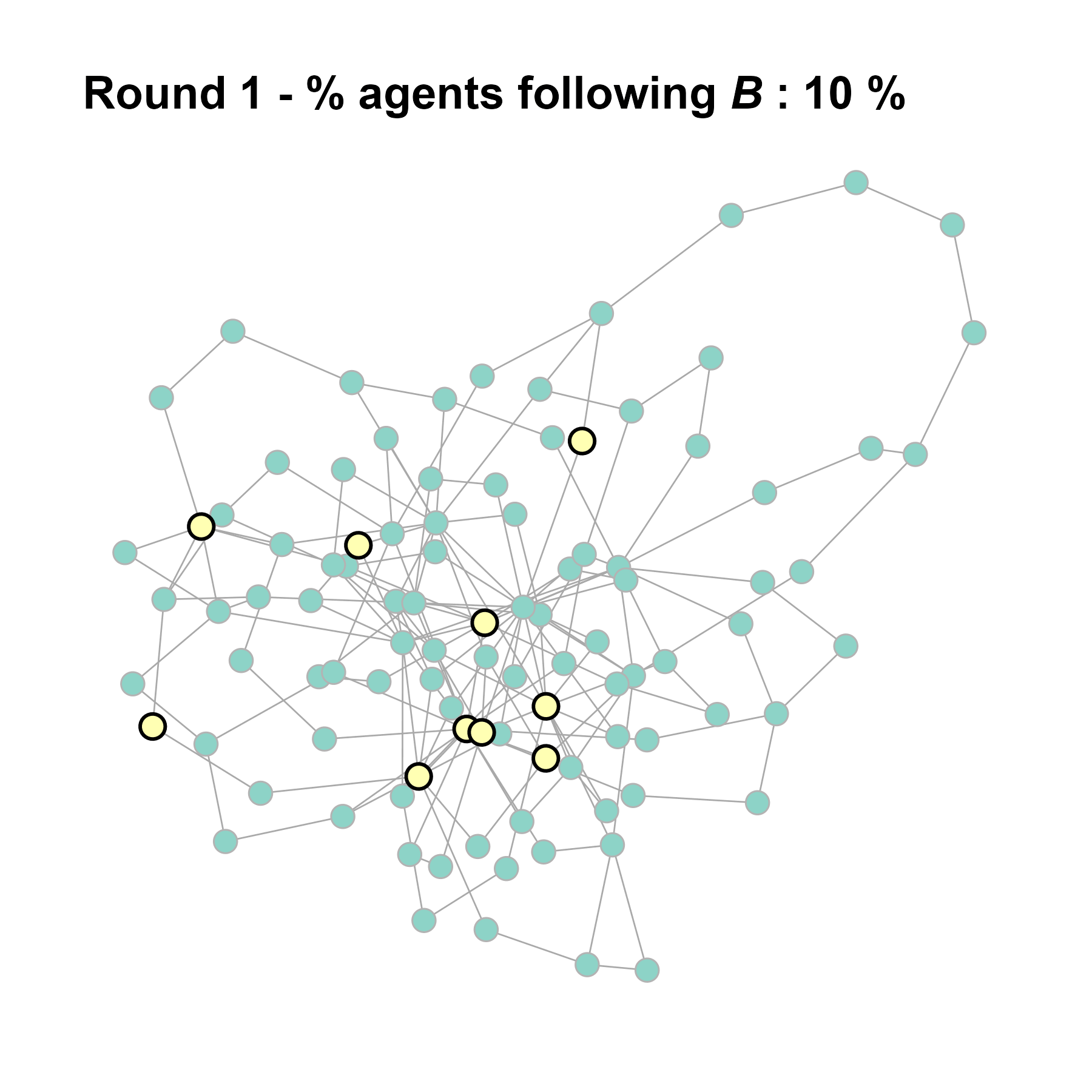

test <- run_one_seed(23, k_min = 2, k_max = 80, alpha = 2.4, rho = 0.4, r = -0.1, return_network = TRUE)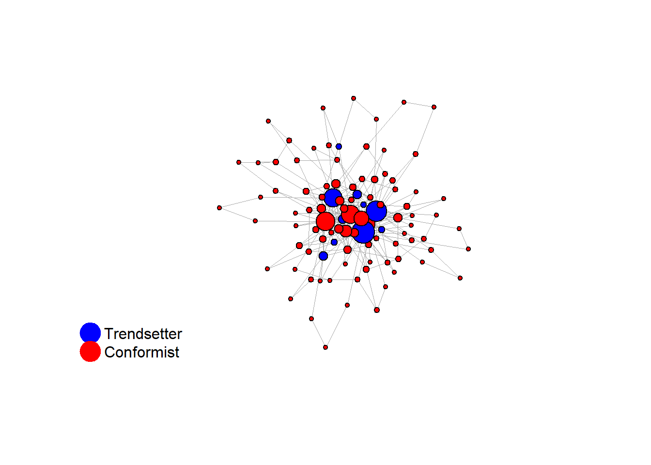

seed = seed + 22
# 22

# 23, 80 #typical s-curve (traction among susceptibles... spraeding in the middle; targeting
# susceptibles not direclty exposed.)

# let's check the distribution of distances to 'trendsetters', among 'conformists'
g <- test$network
trend <- which(V(g)$role == "trendsetter")
conf <- which(V(g)$role == "conformist")

# distances: rows = sources (trendsetters), cols = all vertices
D <- distances(g, v = trend, to = V(g), mode = "all")
Dc <- D[, conf]  #keep just conformists

# calculate (a) the distance to the nearest trendsetter and (b) the average distance to
# trendsetters, across conformists
dists <- data.frame(shortest = apply(Dc, 2, min), average = apply(Dc, 2, function(x) mean(x[is.finite(x)])))
dists_long <- pivot_longer(dists, cols = c(shortest, average), names_to = "type", values_to = "distance_to_seed")

# plot the distribution
ggplot(dists_long, aes(x = distance_to_seed, fill = type)) + geom_histogram(bins = 20, alpha = 0.5, position = "identity") +
    theme_minimal()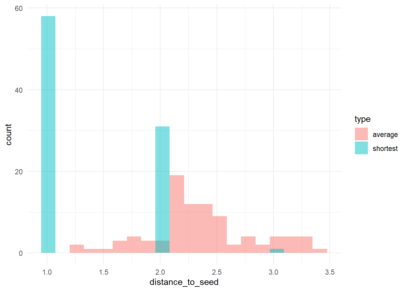

test$stats

#> $run
#> [1] 23
#> 
#> $seed
#> [1] 1253304
#> 
#> $num_nodes
#> [1] 100
#> 
#> $num_edges
#> [1] 268
#> 
#> $avg_degree
#> [1] 5.36
#> 
#> $sd_degree
#> [1] 5.919528
#> 
#> $net_density
#> [1] 0.05414141
#> 
#> $net_diameter
#> [1] 5
#> 
#> $avg_path_len
#> [1] 2.763232
#> 
#> $clust_coeff
#> [1] 0.1984154
#> 
#> $assort_deg
#> [1] -0.1098723
#> 
#> $deg_trait_cor
#> [1] 0.4210629
#> 
#> $components
#> [1] 1

table(degree(test$network))

#> 
#>  2  3  4  5  6  7  9 14 19 22 24 25 28 31 
#> 37 18 12  9  4  2 10  1  1  1  2  1  1  1

# identify trendsetters
ids <- which(V(test$network)$role == "trendsetter")

# check their centrality
sort(as.numeric(cbind(degree(test$network), V(test$network)$role)[ids]))

#>  [1]  4  4  5  5  9  9  9 24 28 31

knitr::include_graphics(paste0("./figures/animation_network_", seed, ".gif"))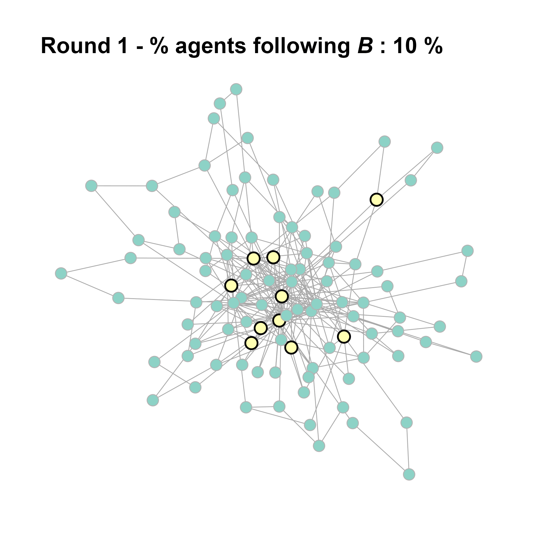

# use this as the network structure for an otree session:
# cbind(degree(test$network),V(test$network)$role)

# convert to adjacency matrix
adj_matrix <- as.matrix(as_adjacency_matrix(test$network))

# get roles
role_vector <- ifelse(V(test$network)$role == "trendsetter", 1, 0)
# create a list to store the network data
net <- list(adj_matrix = adj_matrix, role_vector = role_vector)
# save the list as a JSON file
write_json(net, "network_test_n100.json")

test <- run_one_seed(3, k_min = 2, k_max = 20, alpha = 2.4, rho = 0.4, r = -0.1)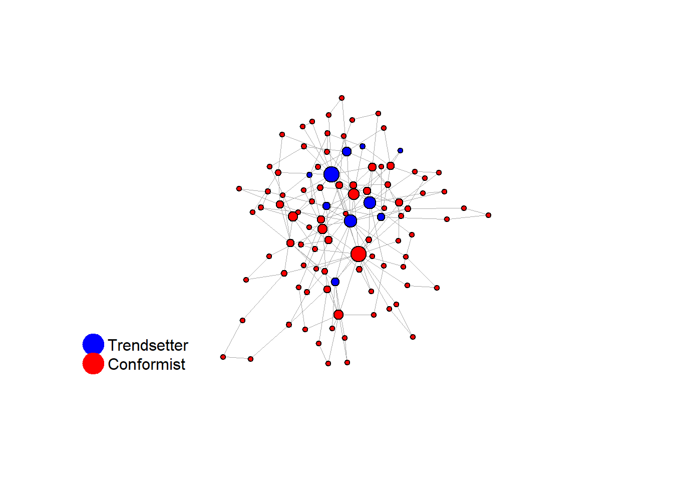

seed = seed - 21
seed = seed + 1

knitr::include_graphics(paste0("./figures/animation_network_", seed, ".gif"))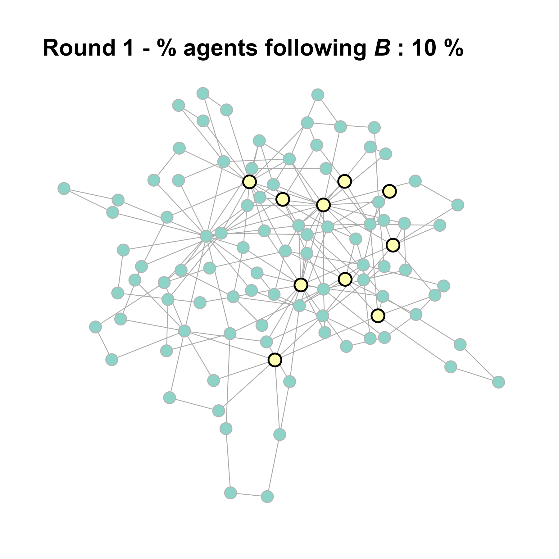

test <- run_one_seed(4, k_min = 2, k_max = 20, alpha = 2.4, rho = 0.4, r = -0.1)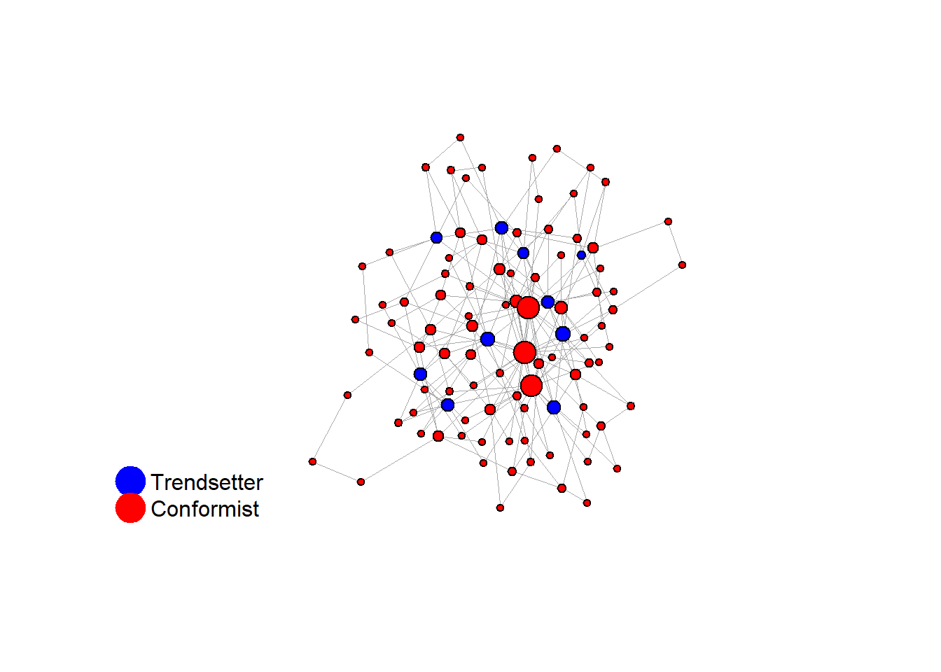

seed = seed + 1

knitr::include_graphics(paste0("./figures/animation_network_", seed, ".gif"))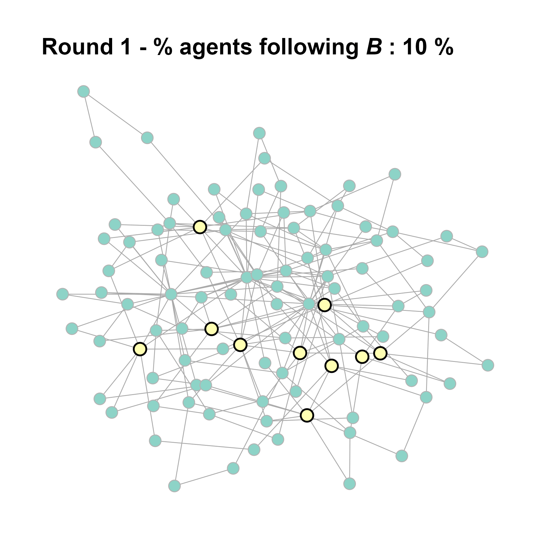

test <- run_one_seed(5, k_min = 2, k_max = 20, alpha = 2.4, rho = 0.4, r = -0.1)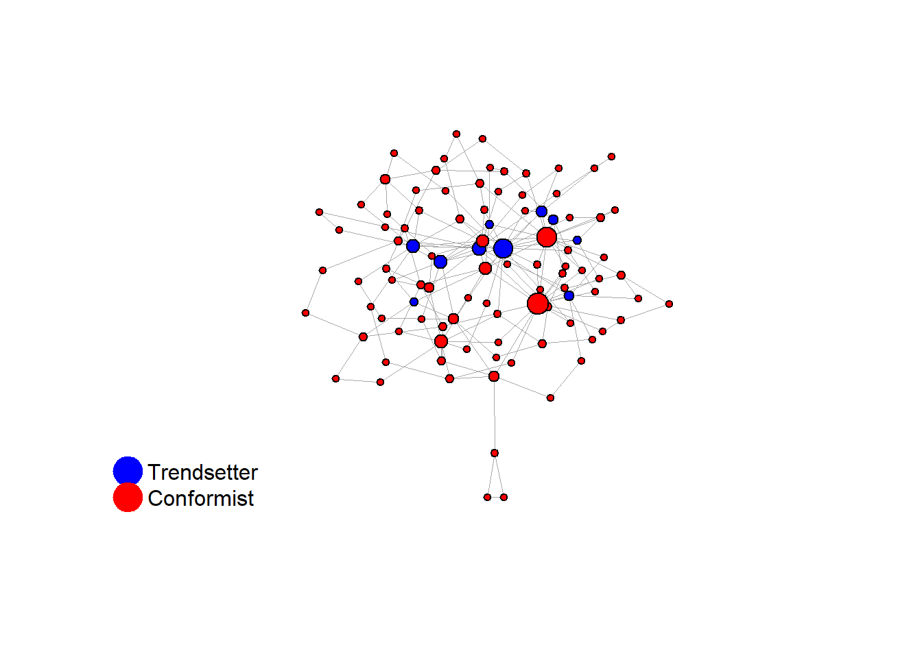

seed = seed + 1

knitr::include_graphics(paste0("./figures/animation_network_", seed, ".gif"))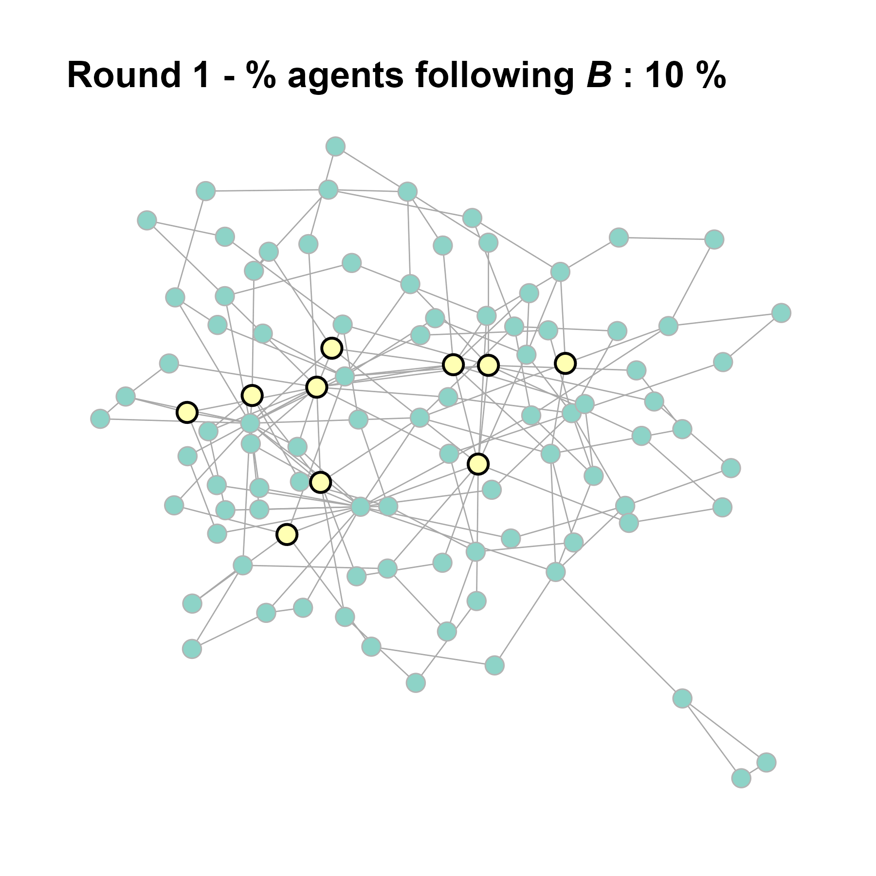

test <- run_one_seed(6, k_min = 2, k_max = 20, alpha = 2.4, rho = 0.4, r = -0.1)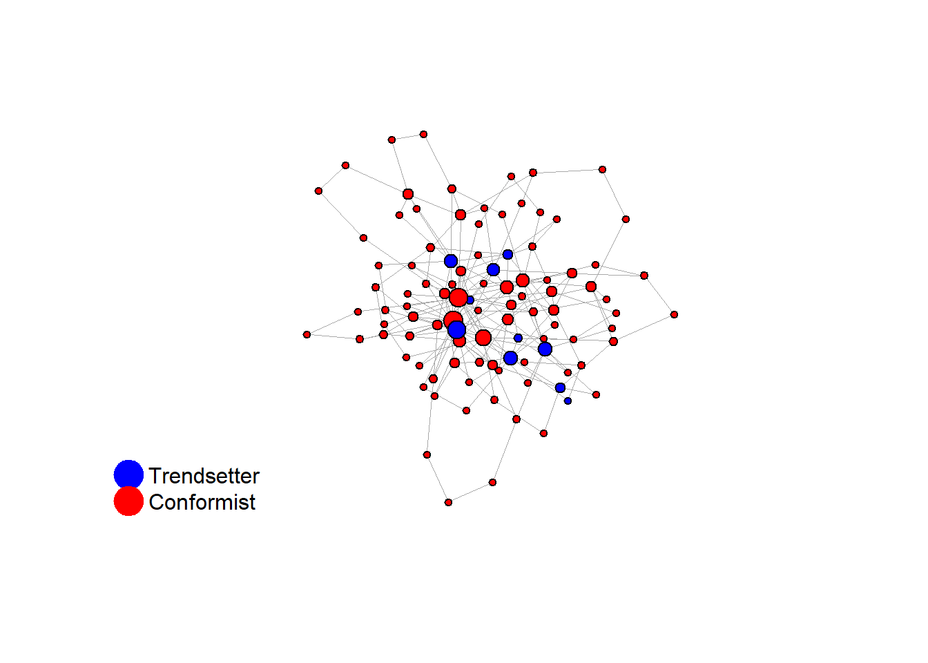

seed = seed + 1

knitr::include_graphics(paste0("./figures/animation_network_", seed, ".gif"))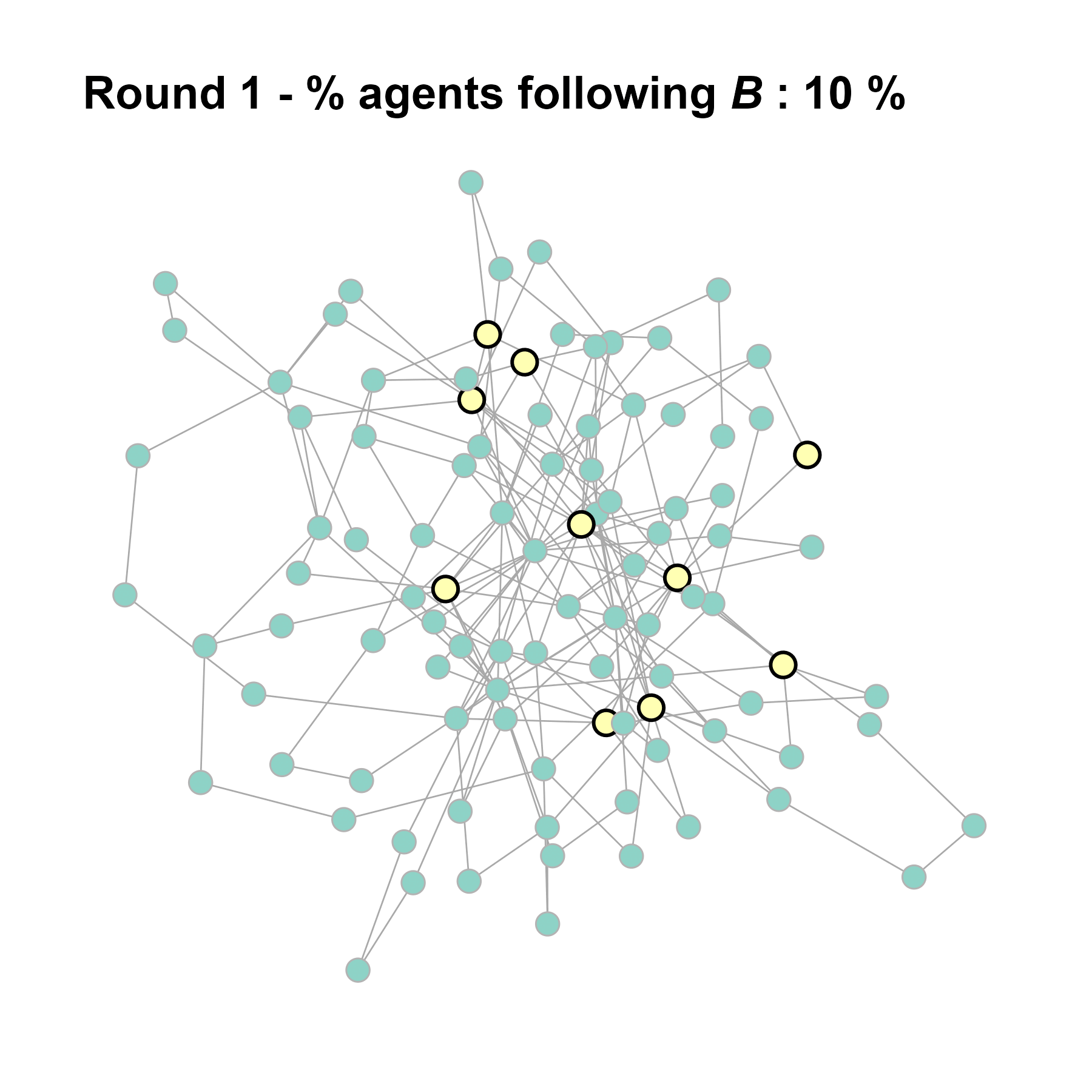

test <- run_one_seed(7, k_min = 2, k_max = 20, alpha = 2.4, rho = 0.4, r = -0.1)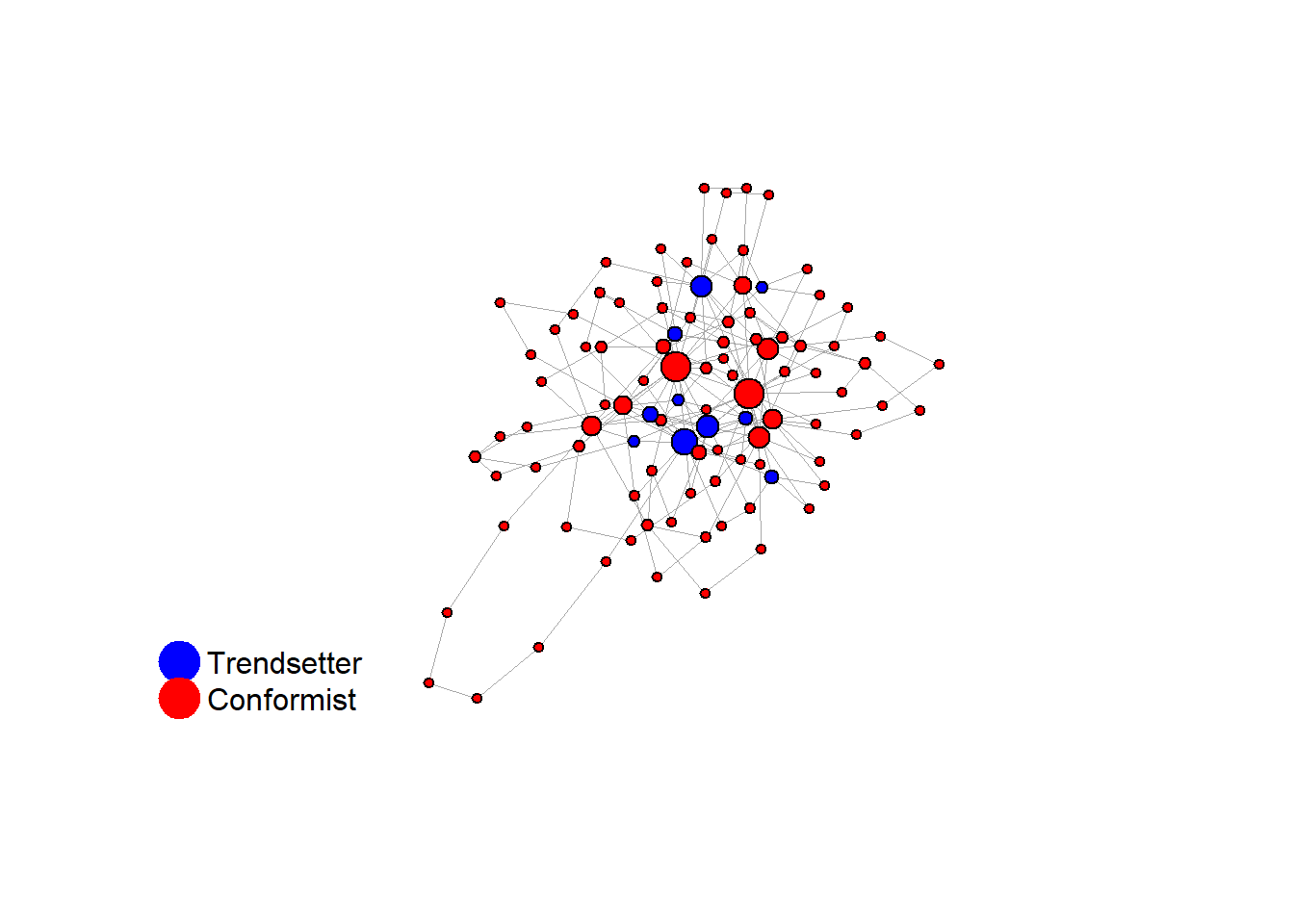

seed = seed + 1

knitr::include_graphics(paste0("./figures/animation_network_", seed, ".gif"))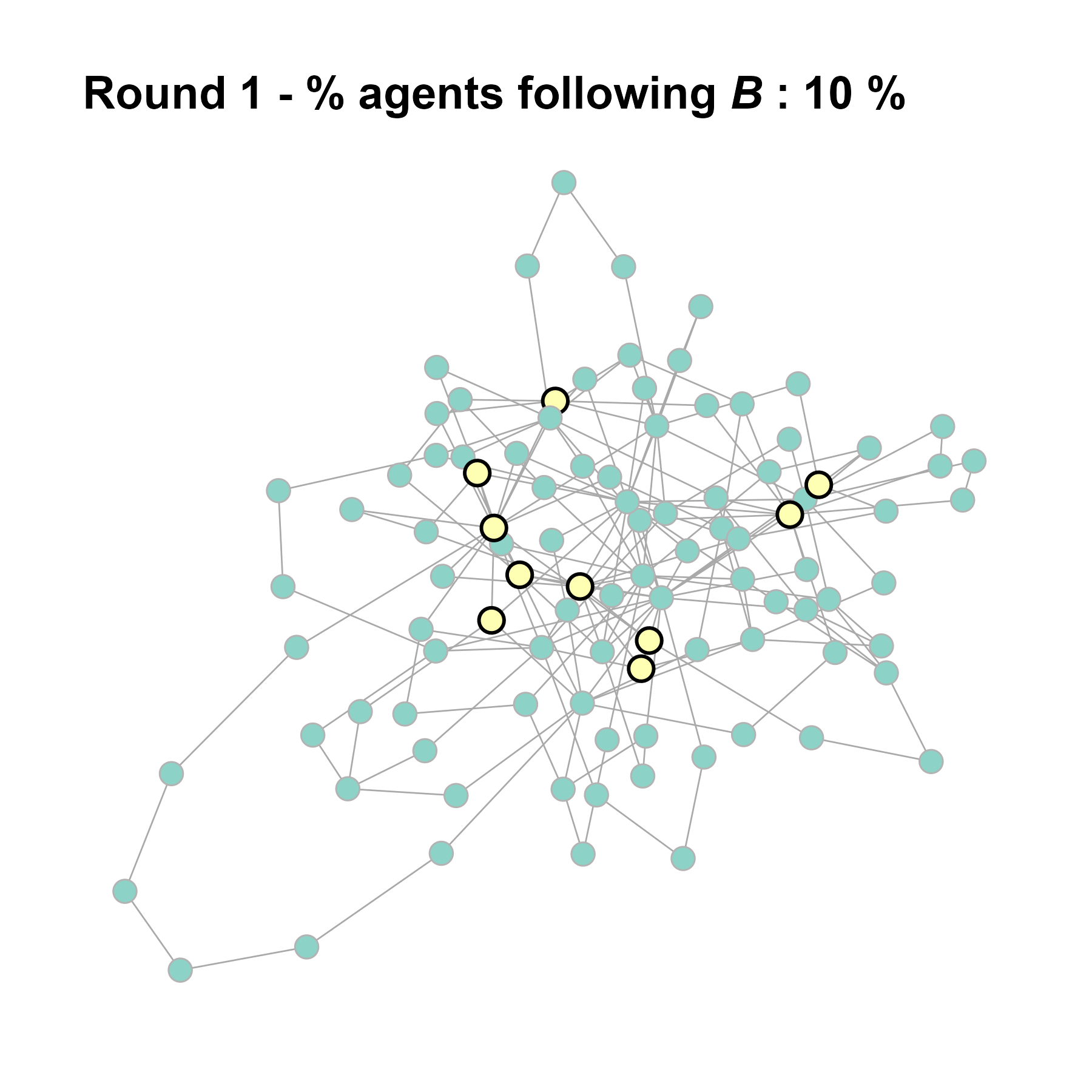

Increase the density:

test <- run_one_seed(8, k_min = 4, k_max = 99, alpha = 2.1, rho = 0.5, r = -0.4)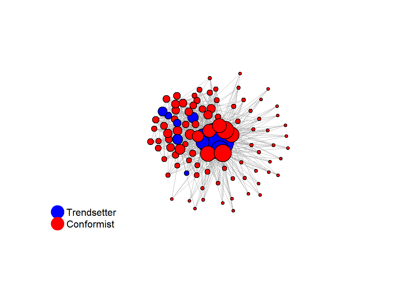

seed = seed + 1

knitr::include_graphics(paste0("./figures/animation_network_", seed, ".gif"))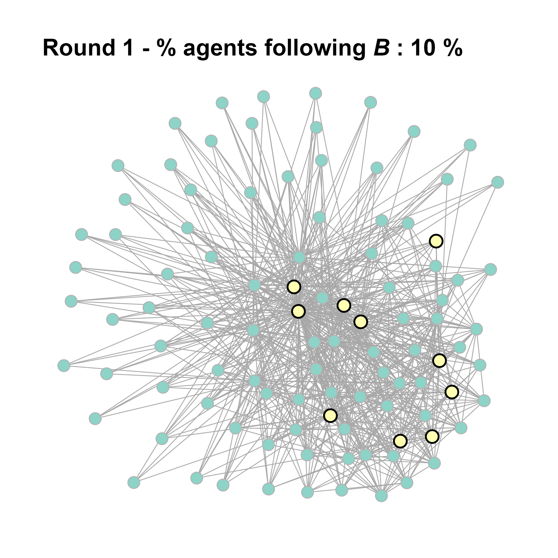

test <- run_one_seed(9, k_min = 4, k_max = 99, alpha = 2.1, rho = 0.5, r = -0.4)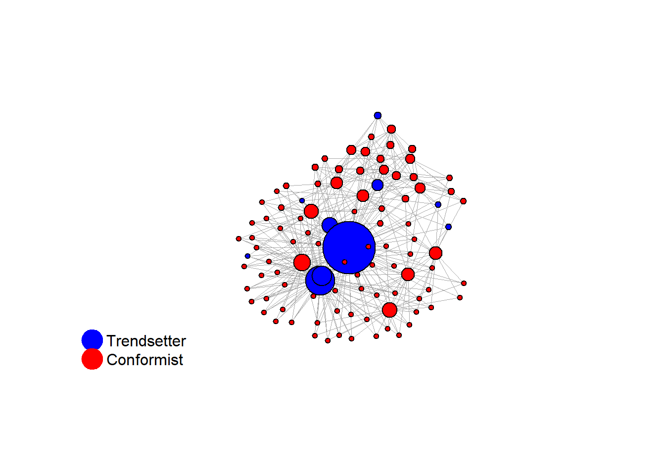

seed = seed + 1

knitr::include_graphics(paste0("./figures/animation_network_", seed, ".gif"))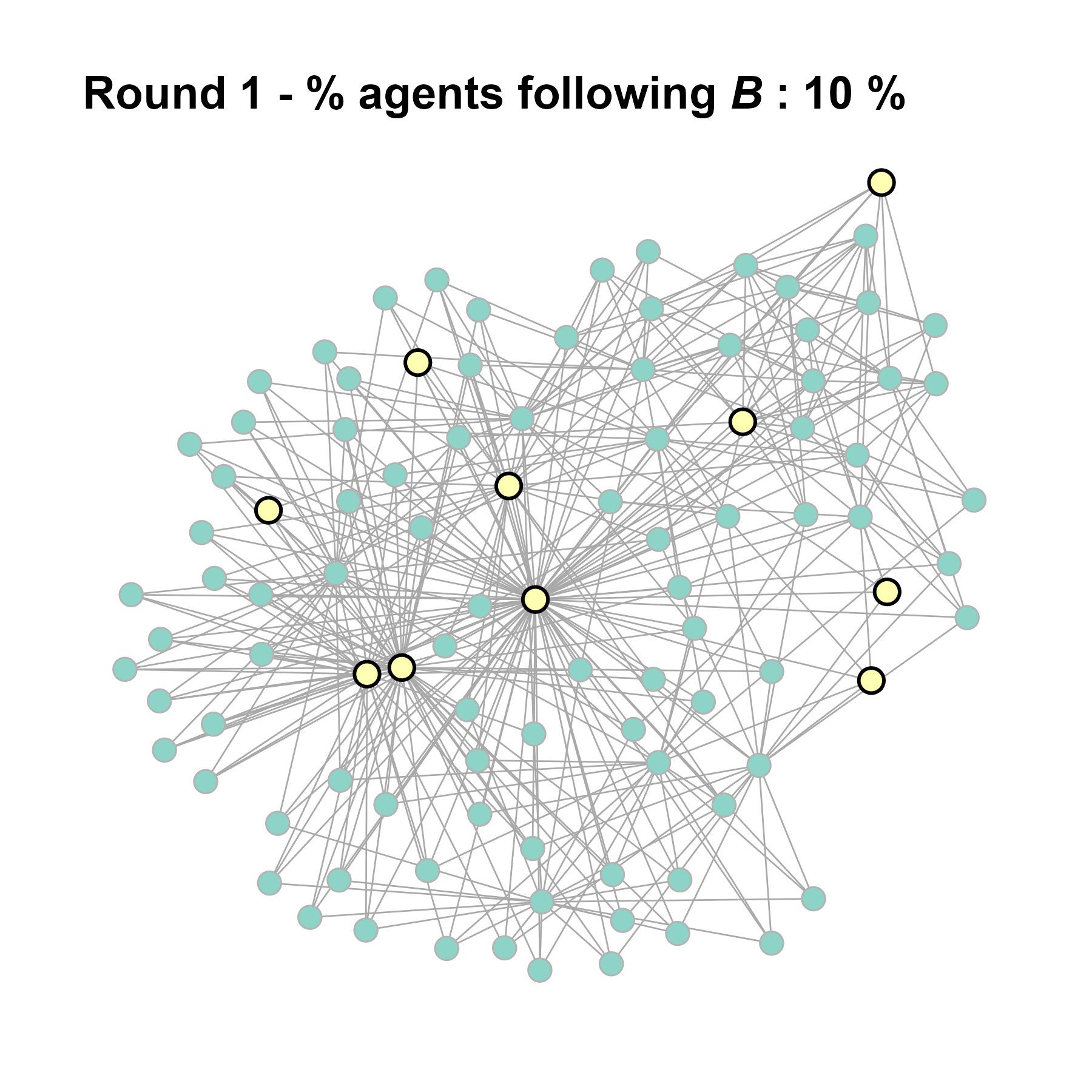

test <- run_one_seed(10, k_min = 4, k_max = 99, alpha = 2.1, rho = 0.5, r = -0.4)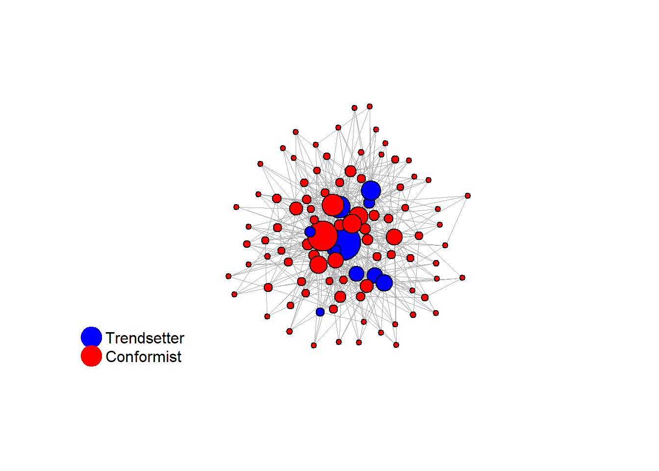

seed = seed + 1

knitr::include_graphics(paste0("./figures/animation_network_", seed, ".gif"))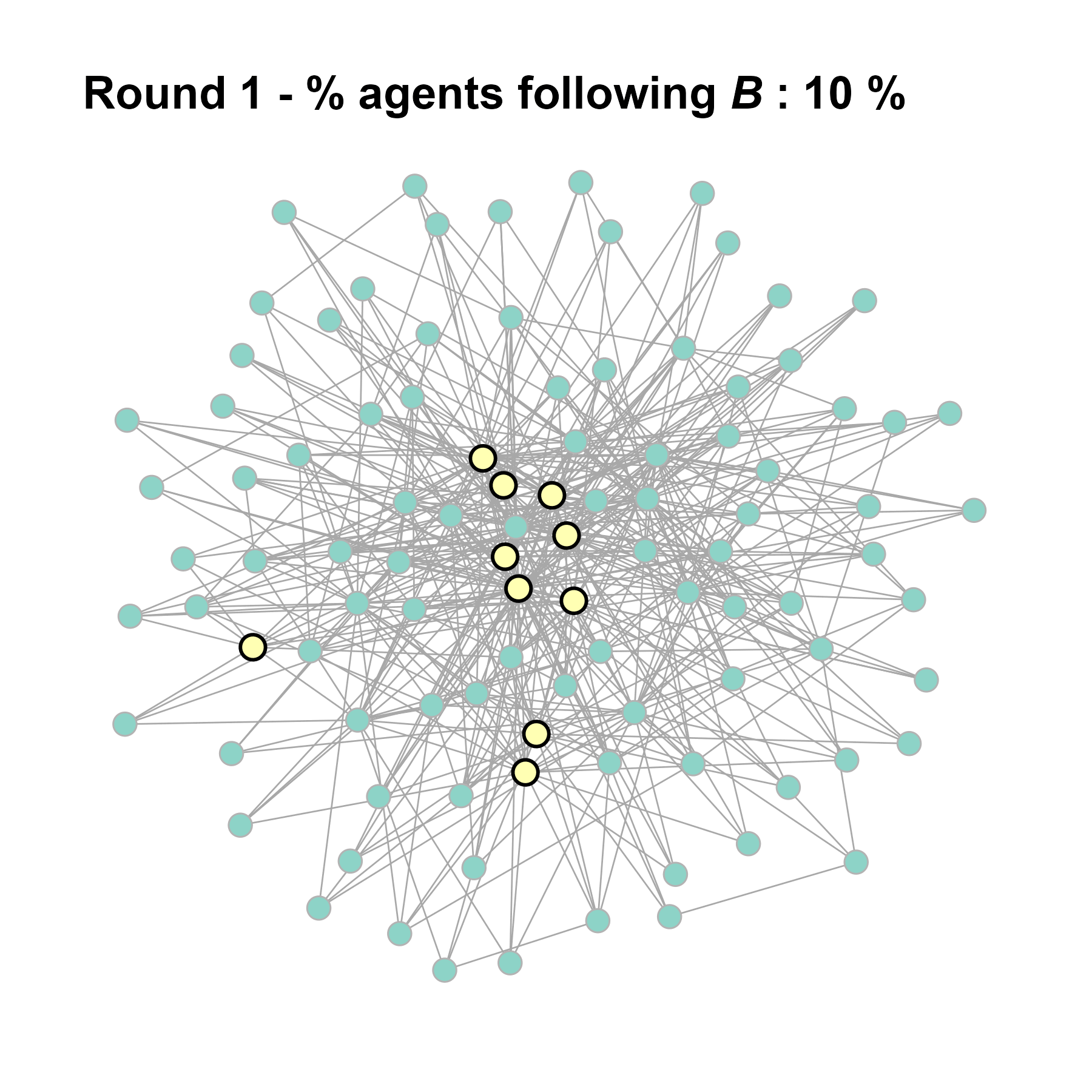

test <- run_one_seed(11, k_min = 4, k_max = 99, alpha = 2.1, rho = 0.5, r = -0.4)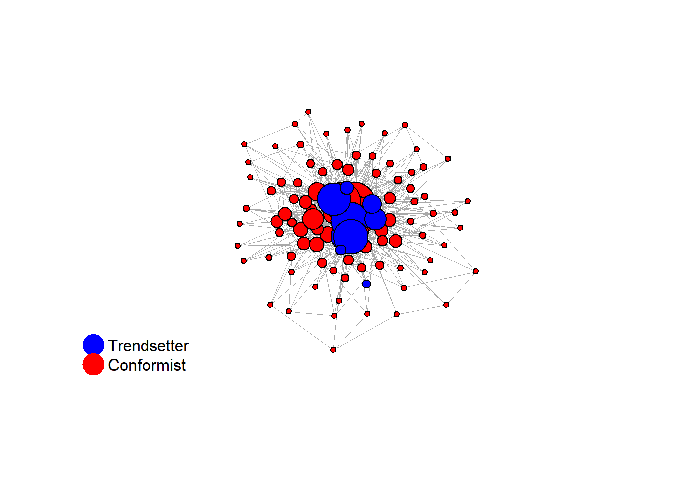

seed = seed + 1

knitr::include_graphics(paste0("./figures/animation_network_", seed, ".gif"))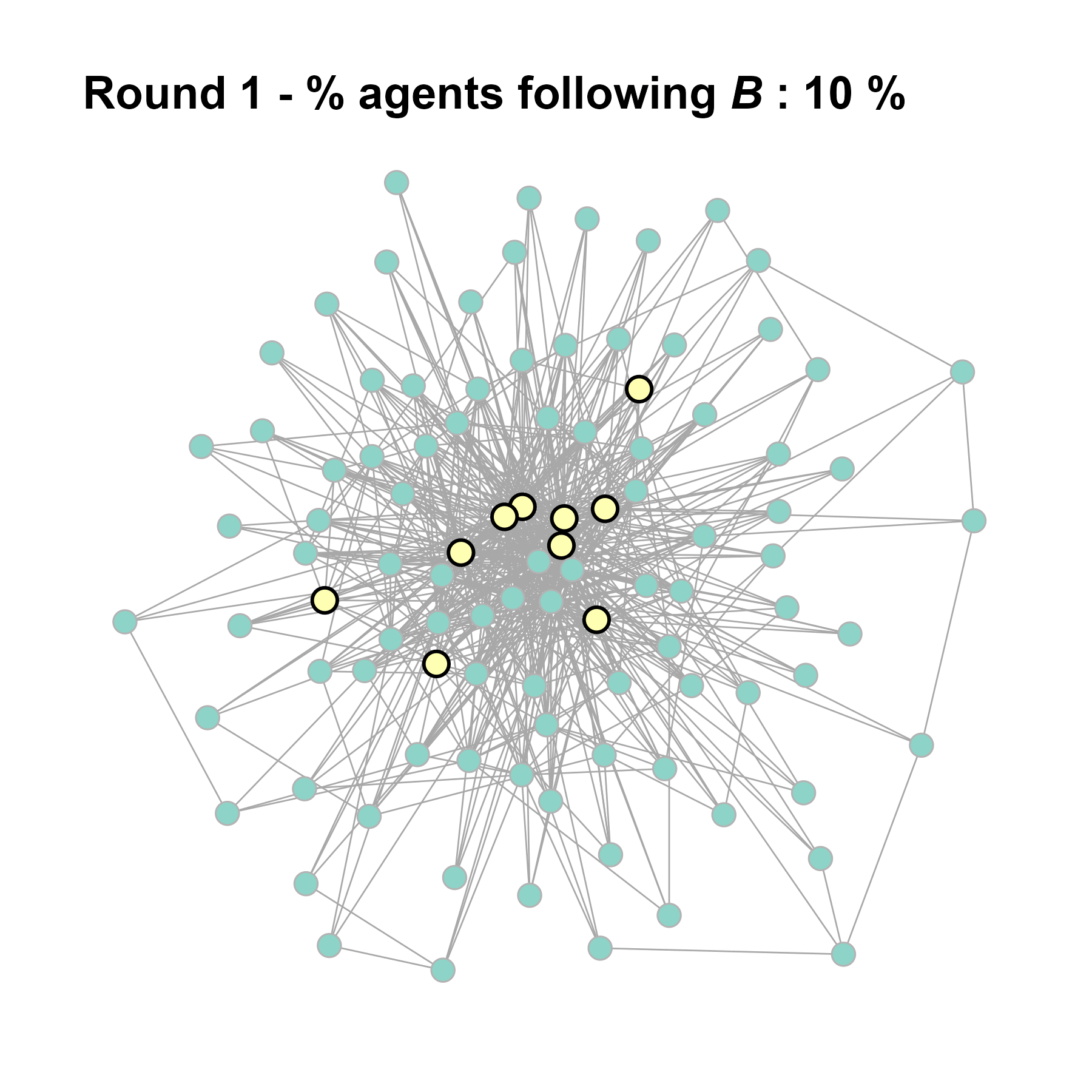

test <- run_one_seed(12, k_min = 4, k_max = 99, alpha = 2.1, rho = 0.5, r = -0.4)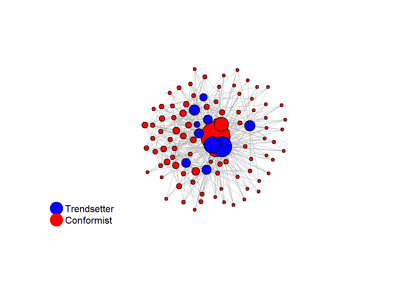

seed = seed + 1

knitr::include_graphics(paste0("./figures/animation_network_", seed, ".gif"))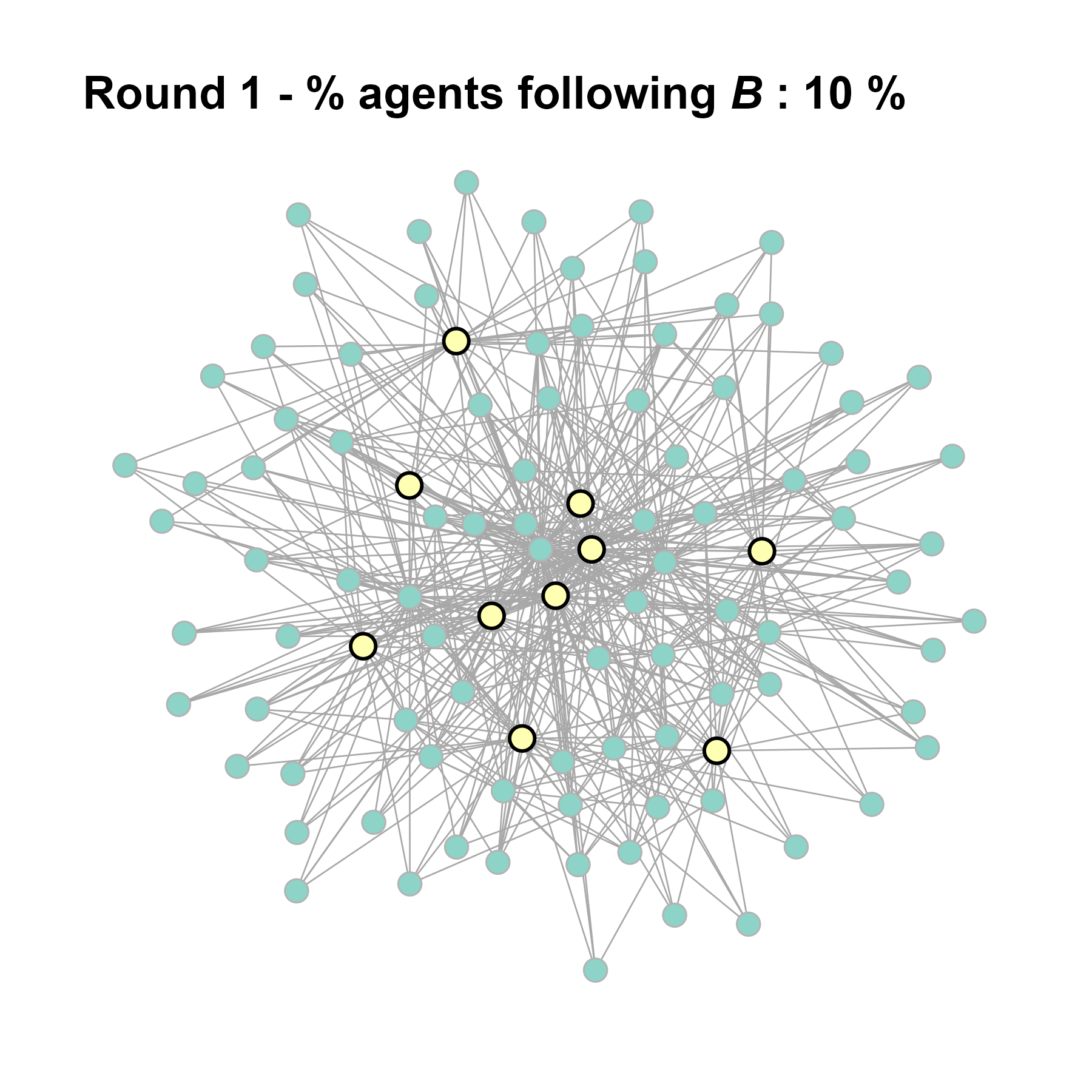

test <- run_one_seed(13, k_min = 4, k_max = 99, alpha = 2.1, rho = 0.5, r = -0.4)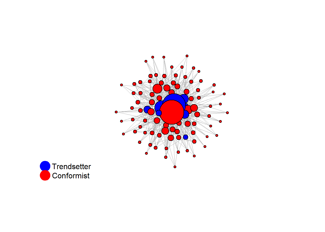

seed = seed + 1

knitr::include_graphics(paste0("./figures/animation_network_", seed, ".gif"))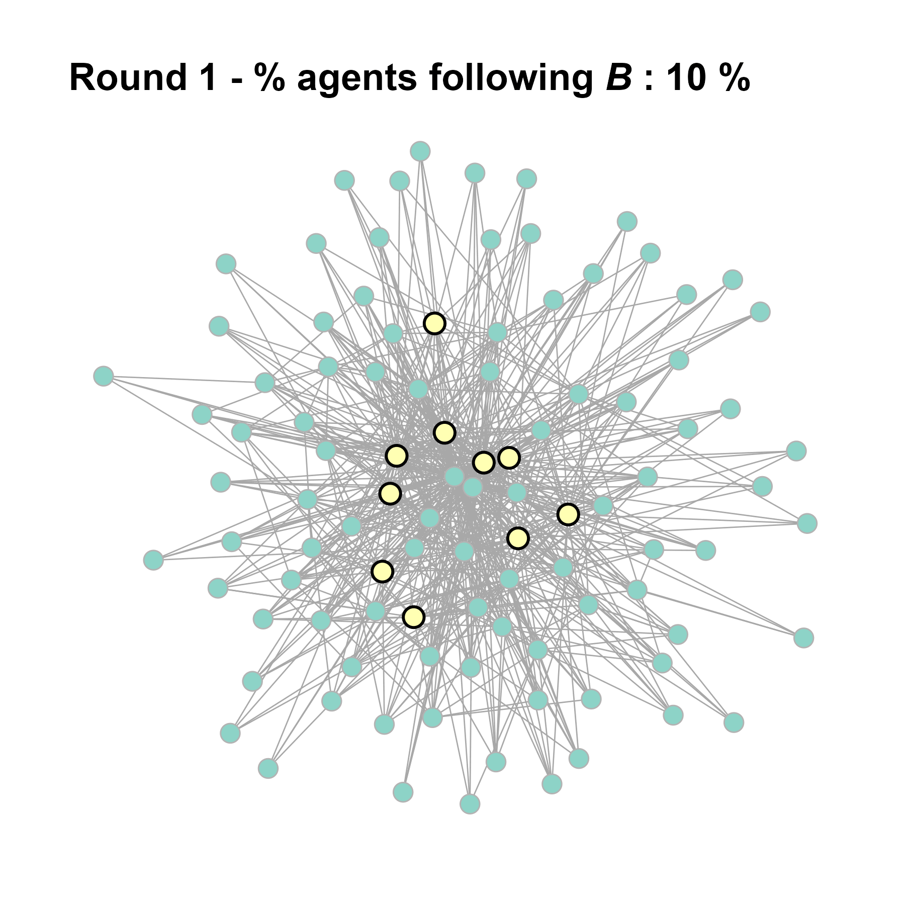

test <- run_one_seed(14, k_min = 4, k_max = 99, alpha = 2.1, rho = 0.5, r = -0.4)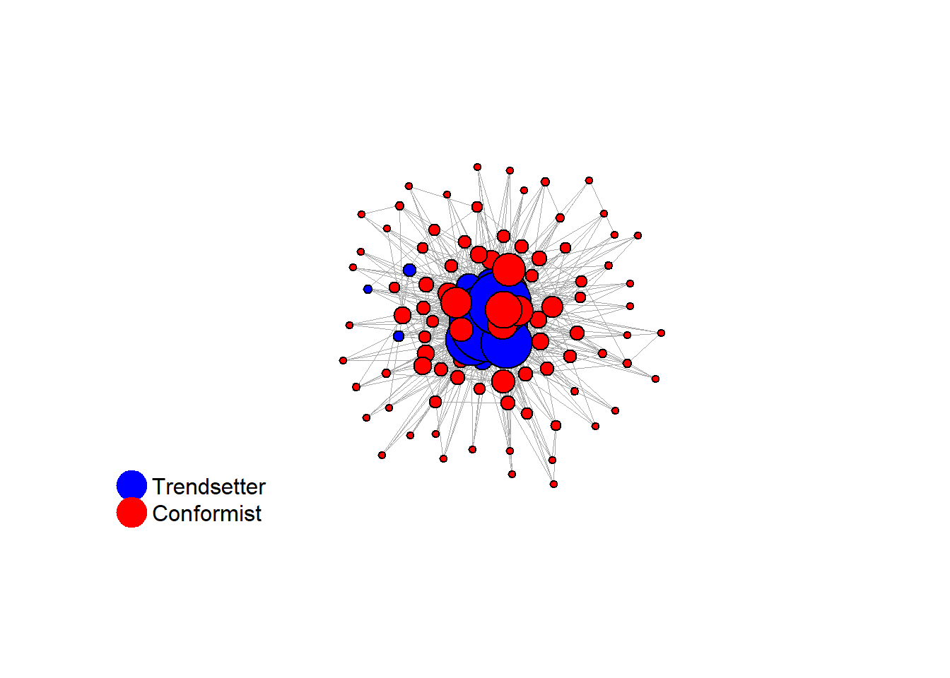

seed = seed + 1

knitr::include_graphics(paste0("./figures/animation_network_", seed, ".gif"))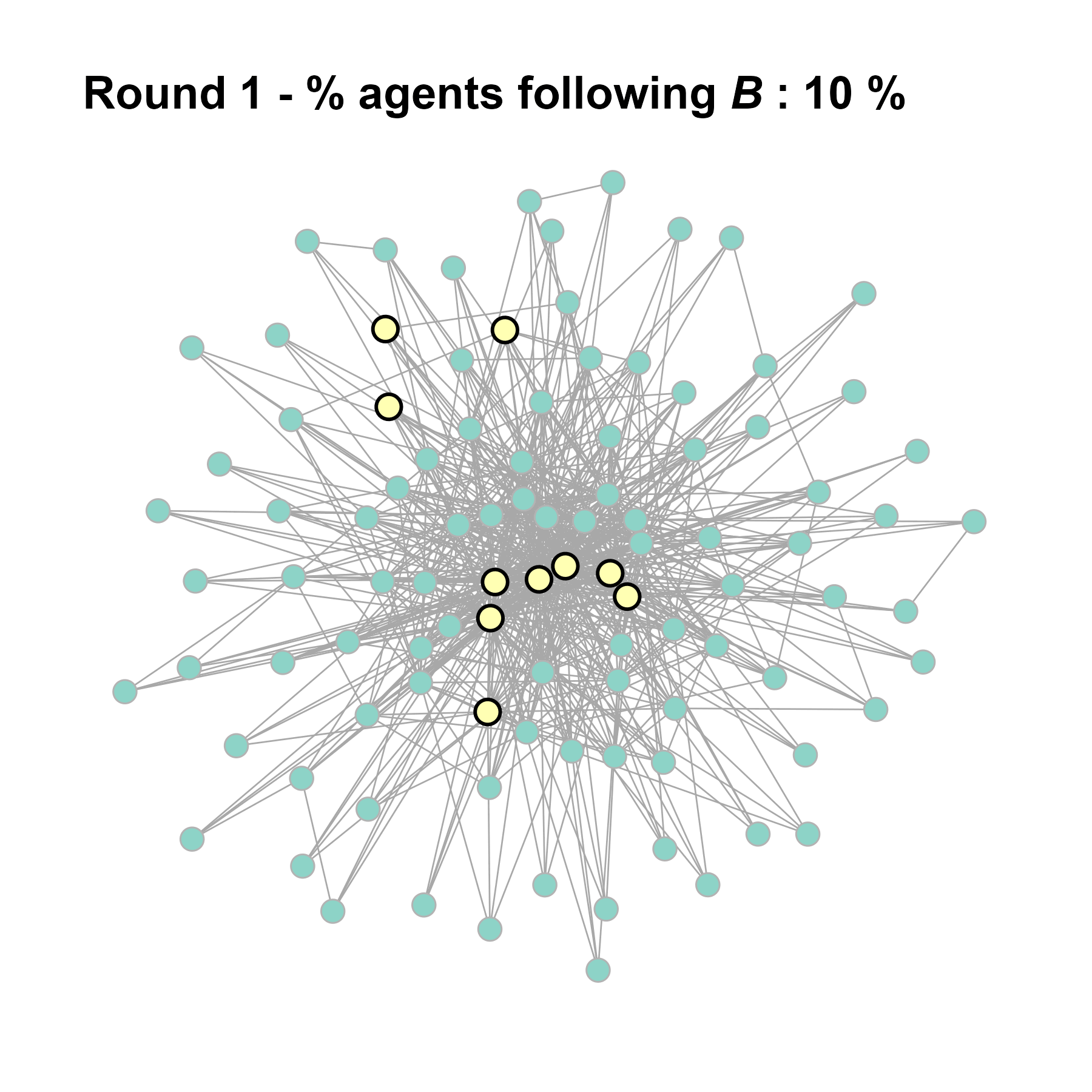

2.2 2. small-worlds

run_one_sw <- function(
  i,
  base_seed = 1253281,
  model = "watts-strogatz",
  beta = 0,
  nei = 3,
  clique_size = 5,
  pmin = 0.1,
  
  params = list(s = 15, e = 10, w = 40, z = 50, lambda1 = 5, lambda2 = 1.8),
  
  # retrieve network
  return_network = FALSE
  
) {
  # derived seed for this run
  seed_i <- base_seed + i
  set.seed(seed_i)

  if (model == "watts-strogatz") {
    network <- sample_smallworld(dim = 1, size = 100, nei = 3, p = beta) }
  else if (model == "caveman") {
    network <- simulate_caveman(n = 100, clique_size = clique_size) 
  }

  V(network)$role <- sample(
    c(rep("trendsetter", round(100*pmin)), rep("conformist", 100-round(100*pmin)))
  )
  
  
  final_network <- network

  
  # --- stats ---
  stats <- list(
    run           = i,
    seed          = seed_i,
    num_nodes     = vcount(final_network),
    num_edges     = ecount(final_network),
    avg_degree    = mean(degree(final_network)),
    sd_degree     = sd(degree(final_network)),
    net_density   = edge_density(final_network),
    net_diameter  = diameter(final_network, directed = FALSE, unconnected = TRUE),
    avg_path_len  = average.path.length(final_network, directed = FALSE),
    clust_coeff   = transitivity(final_network, type = "global"),
    assort_deg    = assortativity_degree(final_network),
    deg_trait_cor = fdegtraitcor(final_network)$cor,
    components    = components(final_network)$no
  )
  
  stats_df <- data.frame(
    Metric = names(stats),
    Value  = unlist(stats),
    row.names = NULL
  )
  
  #print(stats_df)
  fplot_graph(final_network, layout = layout.kamada.kawai(final_network))
  

  # --- initial actions ---
  V(final_network)$action <- ifelse(V(final_network)$role == "trendsetter", 1, 0)
  
  # --- deterministic simulation ---
  sim_det <- fabm(
    network      = final_network,
    params       = params,
    max_rounds   = 50,
    mi_threshold = 0.49,
    choice_rule  = "deterministic",
    plot         = TRUE,
    histories    = TRUE
  )

  # generate the gif for the current network
  gif_filename <- paste0("./figures/animation_network_", seed_i, ".gif")
  gif_path <- fnetworkgif(final_network, sim_det$decision_history, rounds = sim_det$equilibrium$round, output_dir = "./figures")
  # rename the gif to match the naming pattern
  file.rename(gif_path, gif_filename)
  
  
  if (!is.null(sim_det$plot)) {
    print(sim_det$plot)
  }
  
  # --- probabilistic simulation ---
  sim_prob <- fabm(
    network                = final_network,
    params                 = params,
    max_rounds             = 100,
    mi_threshold           = 0.49,
    choice_rule            = "probabilistic",
    stable_window          = 8,   # the length of the window of adoption values
    required_stable_rounds = 20, # number of windows needed to declare equilibrium
    plot                   = TRUE
  )
  if (!is.null(sim_prob$plot)) {
    print(sim_prob$plot)
  }
  
  
  result <- list(
    segregation_det  = sim_det$equilibrium$segregation,
    segregation_prob = sim_prob$equilibrium$segregation,
    stats            = stats
  )
  
  if (return_network) {
    result$network <- final_network
  }
  
  result
}

# random
test <- run_one_sw(i = 15, beta = 1, pmin = 0.1, return_network = TRUE)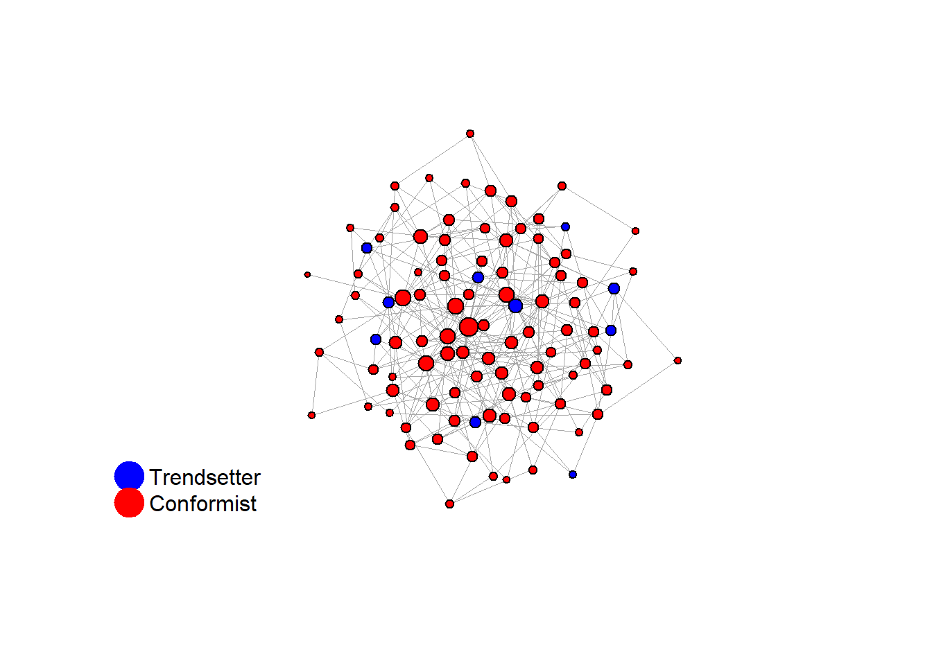

base_seed = 1253281
seed = base_seed + 15

# let's check the distribution of distances to 'trendsetters', among 'conformists'
g <- test$network
trend <- which(V(g)$role == "trendsetter")
conf <- which(V(g)$role == "conformist")

# distances: rows = sources (trendsetters), cols = all vertices
D <- distances(g, v = trend, to = V(g), mode = "all")
Dc <- D[, conf]  #keep just conformists

# calculate (a) the distance to the nearest trendsetter and (b) the average distance to
# trendsetters, across conformists
dists <- data.frame(shortest = apply(Dc, 2, min), average = apply(Dc, 2, function(x) mean(x[is.finite(x)])))
dists_long <- pivot_longer(dists, cols = c(shortest, average), names_to = "type", values_to = "distance_to_seed")

# plot the distribution
ggplot(dists_long, aes(x = distance_to_seed, fill = type)) + geom_histogram(bins = 20, alpha = 0.5, position = "identity") +
    theme_minimal()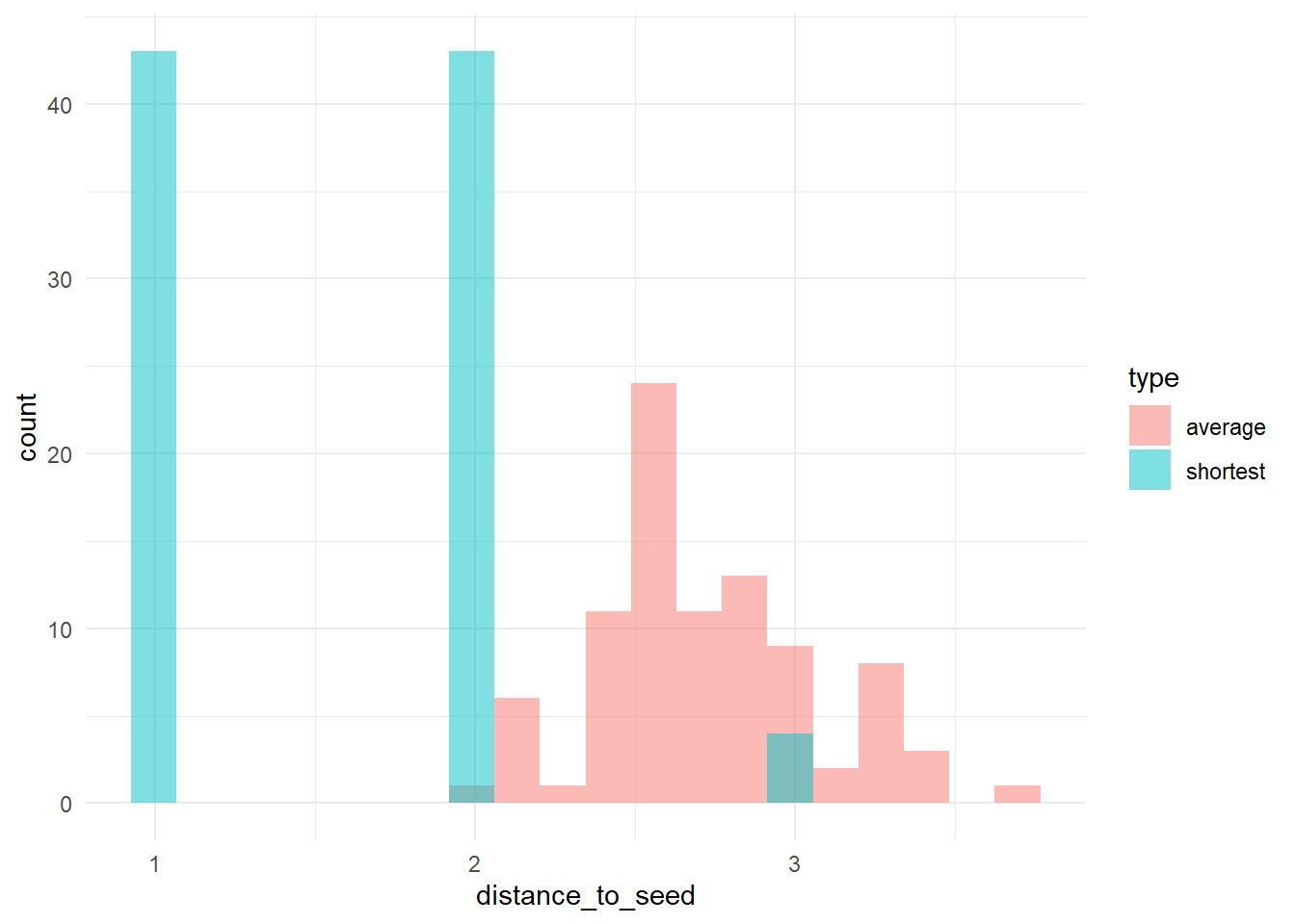

test$stats

#> $run
#> [1] 15
#> 
#> $seed
#> [1] 1253296
#> 
#> $num_nodes
#> [1] 100
#> 
#> $num_edges
#> [1] 300
#> 
#> $avg_degree
#> [1] 6
#> 
#> $sd_degree
#> [1] 2.506557
#> 
#> $net_density
#> [1] 0.06060606
#> 
#> $net_diameter
#> [1] 5
#> 
#> $avg_path_len
#> [1] 2.731919
#> 
#> $clust_coeff
#> [1] 0.05963556
#> 
#> $assort_deg
#> [1] -0.00588506
#> 
#> $deg_trait_cor
#> [1] 0.04009635
#> 
#> $components
#> [1] 1

table(degree(test$network))

#> 
#>  1  2  3  4  5  6  7  8  9 10 11 12 15 
#>  1  4 11 15  9 23 16  7  5  3  3  2  1

# identify trendsetters
ids <- which(V(test$network)$role == "trendsetter")

# check their centrality
sort(as.numeric(cbind(degree(test$network), V(test$network)$role)[ids]))

#>  [1]  3  4  6  6  6  7  7  7  7 10

knitr::include_graphics(paste0("./figures/animation_network_", seed, ".gif"))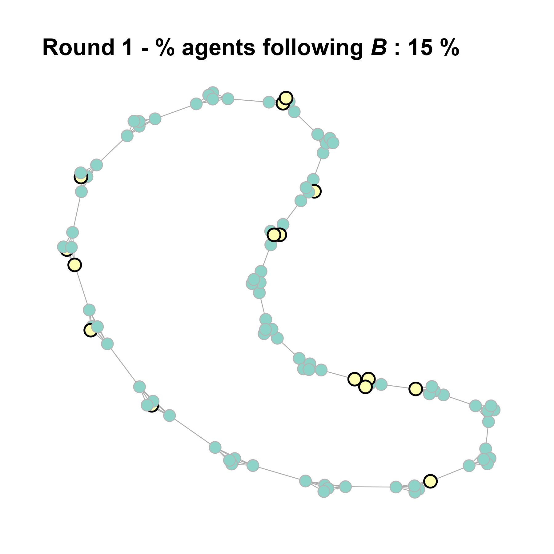

# use this as the network structure for an otree session:
# cbind(degree(test$network),V(test$network)$role)

# convert to adjacency matrix
adj_matrix <- as.matrix(as_adjacency_matrix(test$network))

# get roles
role_vector <- ifelse(V(test$network)$role == "trendsetter", 1, 0)
# create a list to store the network data
net <- list(adj_matrix = adj_matrix, role_vector = role_vector)
# save the list as a JSON file
write_json(net, "network_test_n100_random.json")

test <- run_one_sw(i = 15, model = "caveman", clique_size = 5, pmin = 0.15, return_network = TRUE)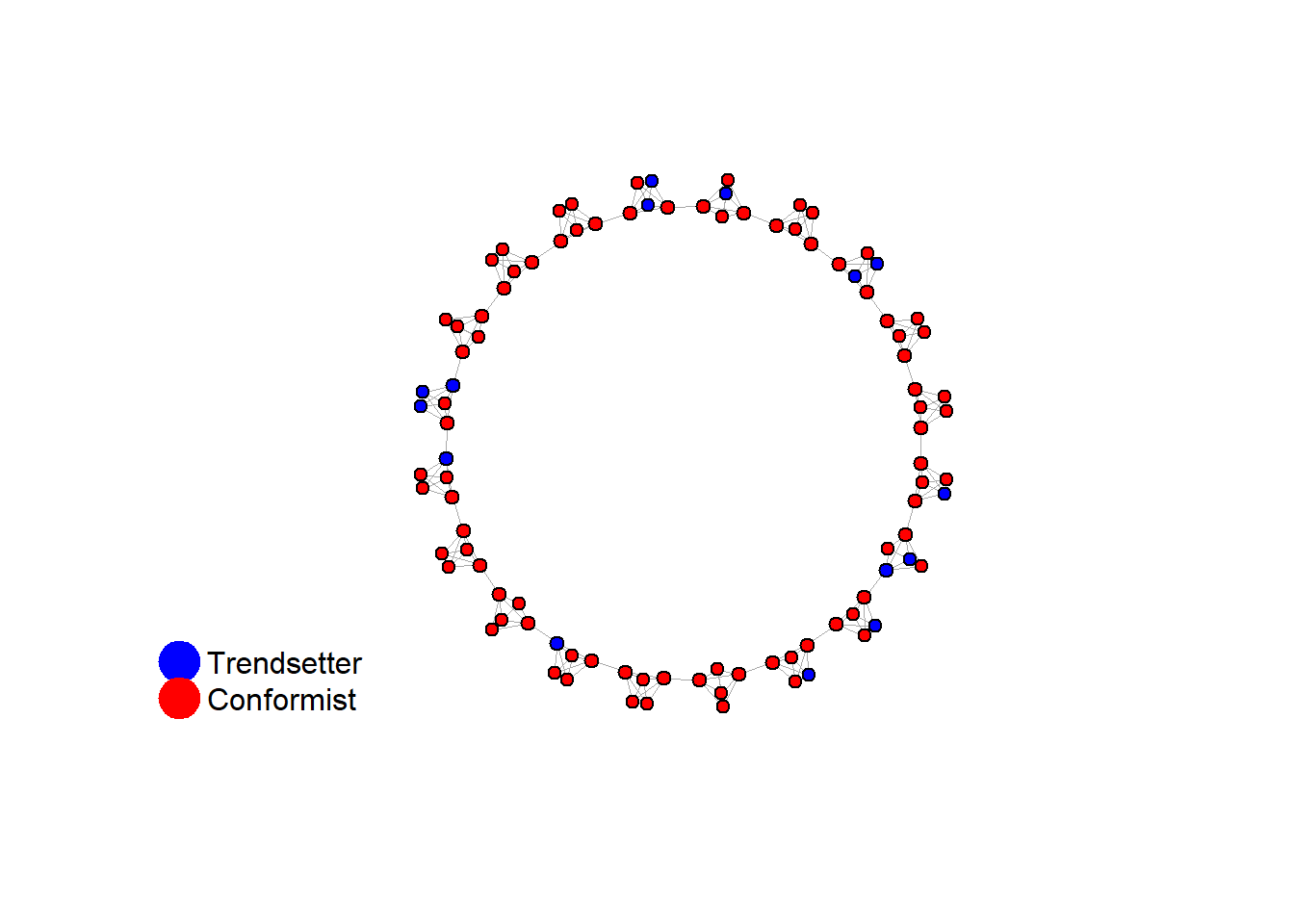

seed = seed + 1

# knitr::include_graphics(paste0('./figures/animation_network_', seed ,'.gif'))

---

Copyright © Rob Franken