Experiment
Last compiled on 23-03-2026
1 Getting started
To copy the code, click the button in the upper right corner of the code-chunks.
1.1 clean up
rm(list = ls())
gc()
1.2 custom functions
We defined a number custom functions, at Download custom_functions.R.
source("./custom_functions.R")1.3 necessary packages
tidyverse: data wranglingigraph: generate and visualize graphsparallel: parallel computing to speed up simulationforeach: looping in paralleldoParallel: parallel backend forforeachggplot2: data visualizationggh4x: hacks forggplot2ggpubr: make visualizations publication-ready
packages = c("tidyverse", "igraph", "ggplot2", "parallel", "doParallel", "foreach", "ggh4x", "ggpubr",
    "plotly", "RColorBrewer", "grid", "gridExtra", "patchwork", "ggplotify", "ggraph", "gganimate", "RColorBrewer",
    "ggtext", "magick", "jsonlite", "lubridate", "ggtext")

invisible(fpackage.check(packages))
rm(packages)
2 Experimental conditions
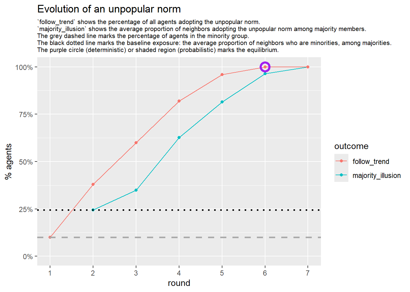
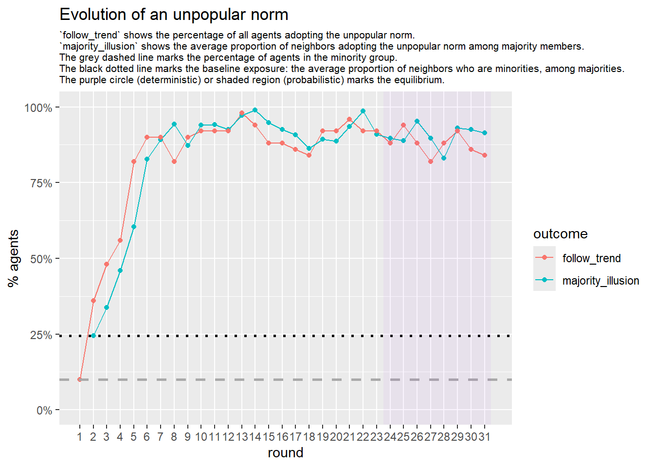
2.1 1. heavy-tailed network with central minorities
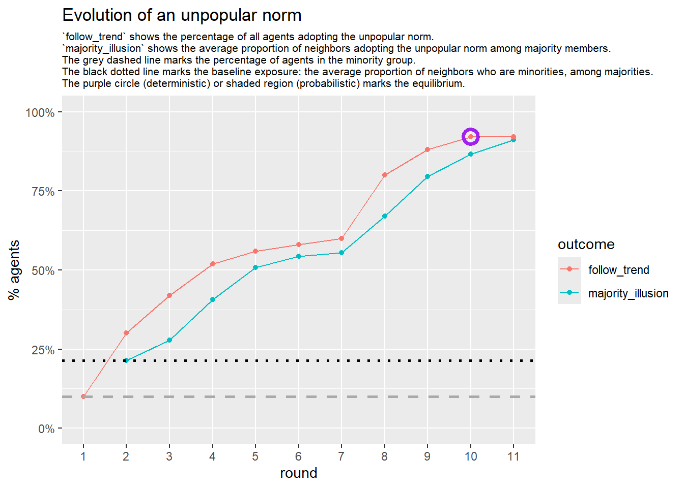
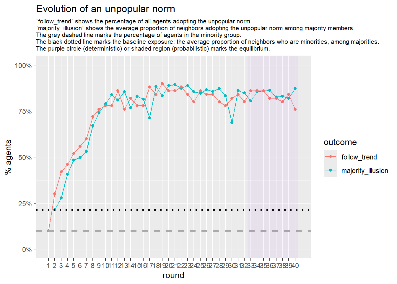
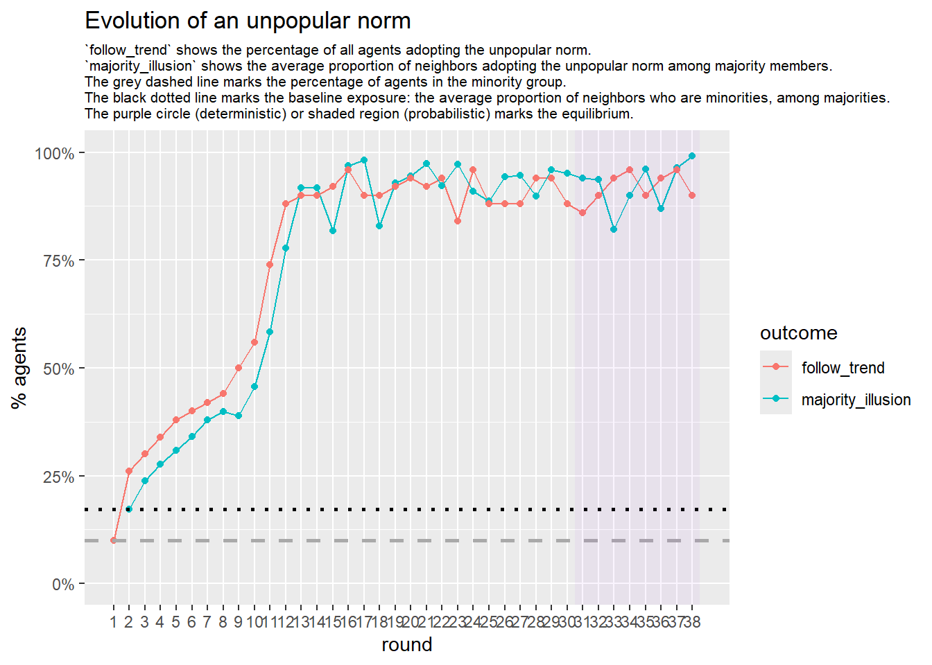
Let’s take a likely-case for an unpopular norm, generate multiple networks of this target, and simulate the emergence of the norm following a deterministic and probabilistic choice model:
# pick one configuration that likely leads to an unpopular norm, and explore multiple 'seeds':
run_one_seed <- function(
i,
base_seed = 2253281,
params = list(s = 15, e = 10, w = 40, z = 50, lambda1 = 5, lambda2 = 1.8),
# tweak network
k_min = 2,
k_max = 20,
alpha = 2.4,
rho = 0.4,
r = -0.1,
# retrieve network
return_network = FALSE
) {
# derived seed for this run
seed_i <- base_seed + i
set.seed(seed_i)
# --- network creation ---
degseq <- fdegseq(
n = 50,
alpha = alpha,
k_min = k_min,
k_max = k_max,
dist = "log-normal", #use log-normal
seed = seed_i
)
network <- sample_degseq(degseq, method = "vl")
V(network)$role <- sample(
c(rep("trendsetter", 5), rep("conformist", 45))
)
rewired_network <- frewire_r(network, r, verbose = FALSE, max_iter = 1e5)
final_network <- fswap_rho(rewired_network, rho, verbose = FALSE, max_iter = 1e4)
# --- stats ---
stats <- list(
run = i,
seed = seed_i,
num_nodes = vcount(final_network),
num_edges = ecount(final_network),
avg_degree = mean(degree(final_network)),
sd_degree = sd(degree(final_network)),
net_density = edge_density(final_network),
net_diameter = diameter(final_network, directed = FALSE, unconnected = TRUE),
avg_path_len = average.path.length(final_network, directed = FALSE),
clust_coeff = transitivity(final_network, type = "global"),
assort_deg = assortativity_degree(final_network),
deg_trait_cor = fdegtraitcor(final_network)$cor,
components = components(final_network)$no
)
fplot_graph(final_network, layout = layout_with_fr(final_network))
# --- initial actions ---
V(final_network)$action <- ifelse(V(final_network)$role == "trendsetter", 1, 0)
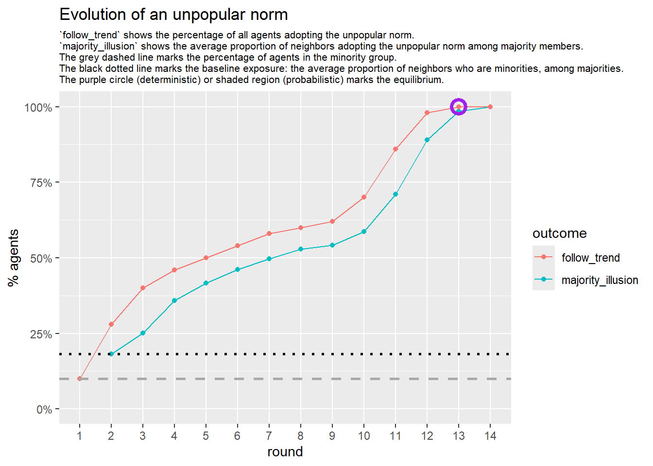
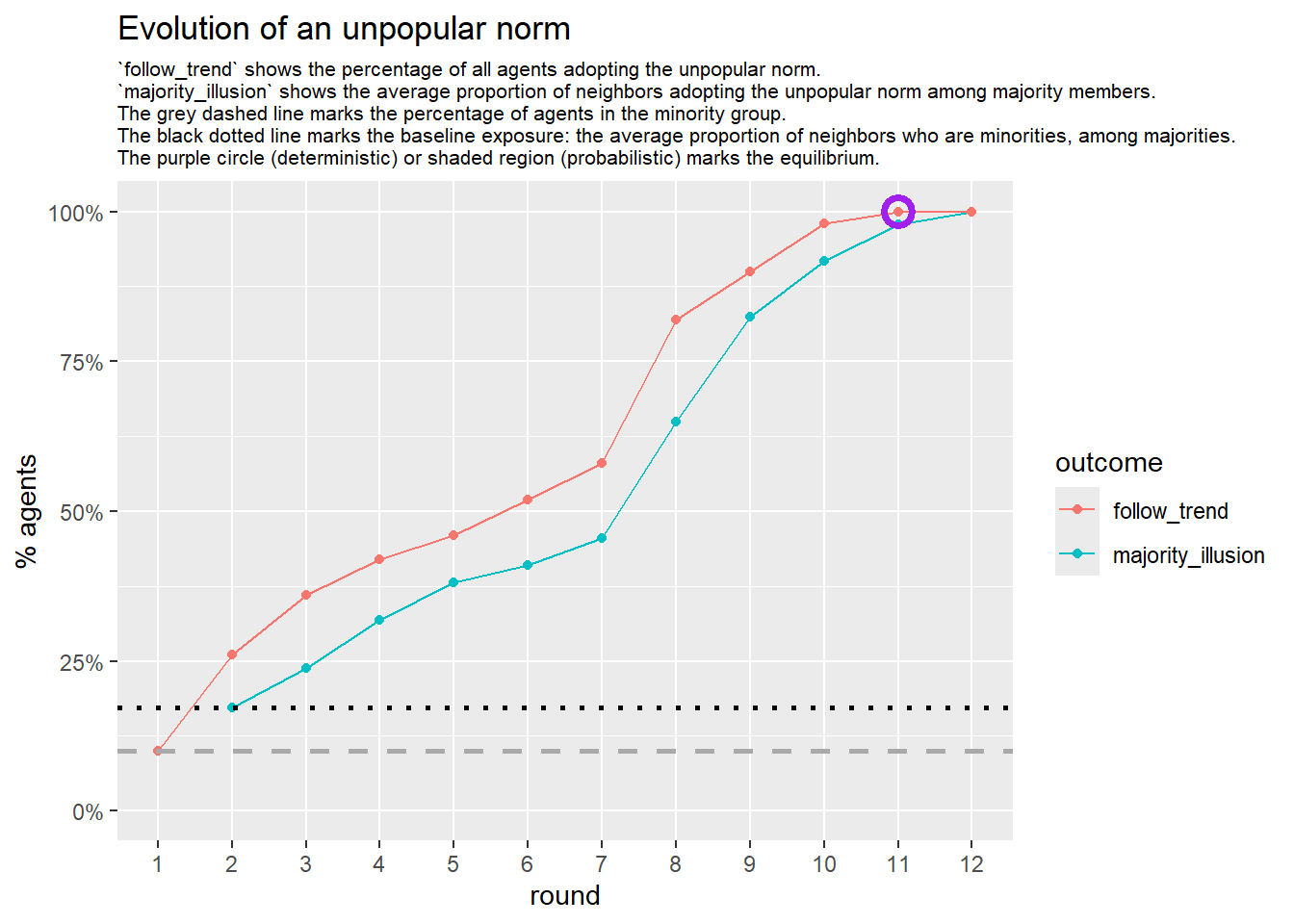
# --- deterministic simulation ---
sim_det <- fabm(
network = final_network,
params = params,
max_rounds = 50,
mi_threshold = 0.49,
choice_rule = "deterministic",
plot = TRUE,
histories = TRUE
)
# generate the gif for the current network
gif_filename <- paste0("./figures/animation_network_", seed_i, ".gif")
gif_path <- fnetworkgif(final_network, sim_det$decision_history, rounds = sim_det$equilibrium$round, output_dir = "./figures")
# rename the gif to match the naming pattern
file.rename(gif_path, gif_filename)
if (!is.null(sim_det$plot)) {
print(sim_det$plot)
}
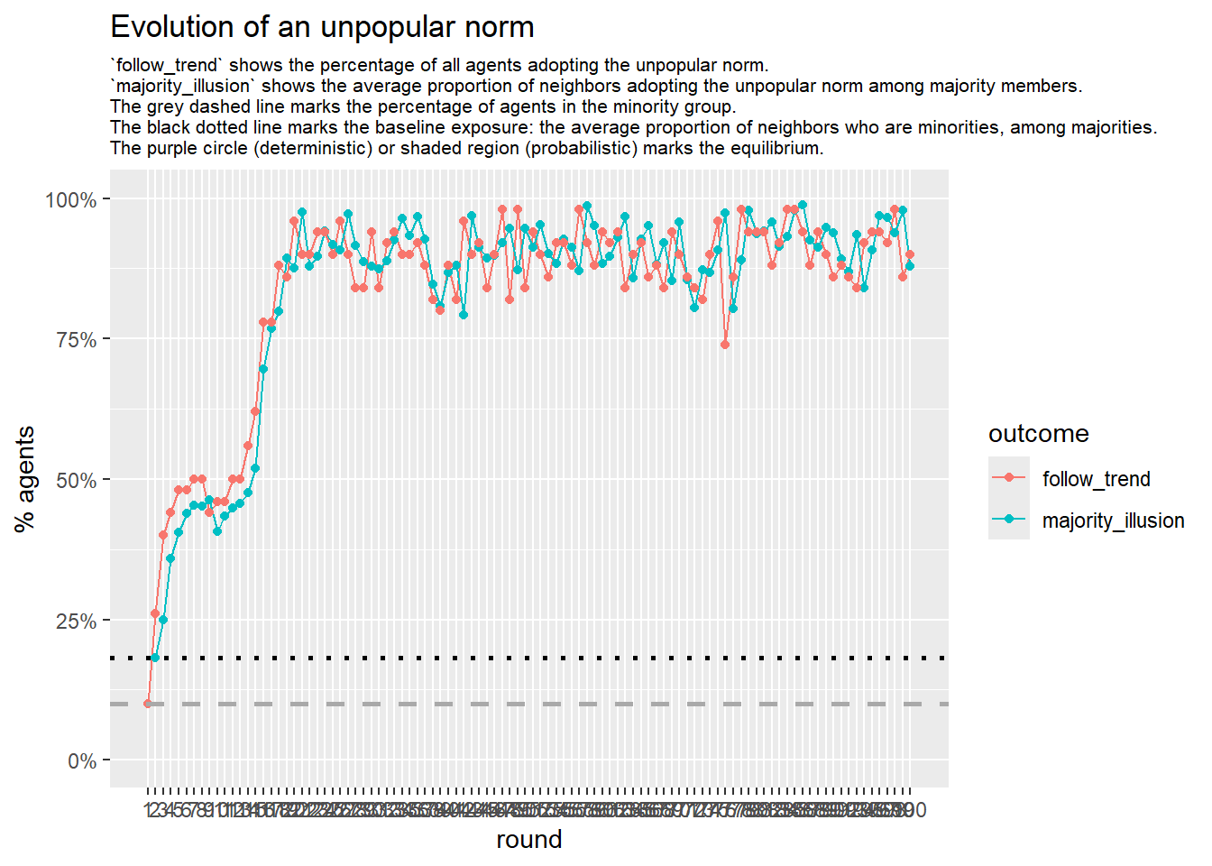
# --- probabilistic simulation ---
sim_prob <- fabm(
network = final_network,
params = params,
max_rounds = 100,
mi_threshold = 0.49,
choice_rule = "probabilistic",
stable_window = 8, # the length of the window of adoption values
required_stable_rounds = 20, # number of windows needed to declare equilibrium
plot = TRUE
)
if (!is.null(sim_prob$plot)) {
print(sim_prob$plot)
}
result <- list(
segregation_det = sim_det$equilibrium$segregation,
segregation_prob = sim_prob$equilibrium$segregation,
stats = stats
)
if (return_network) {
result$network <- final_network
}
result
}test <- run_one_seed(2, k_min = 2, k_max = 20, alpha = 2.4, rho = 0.4, r = -0.1, return_network = TRUE)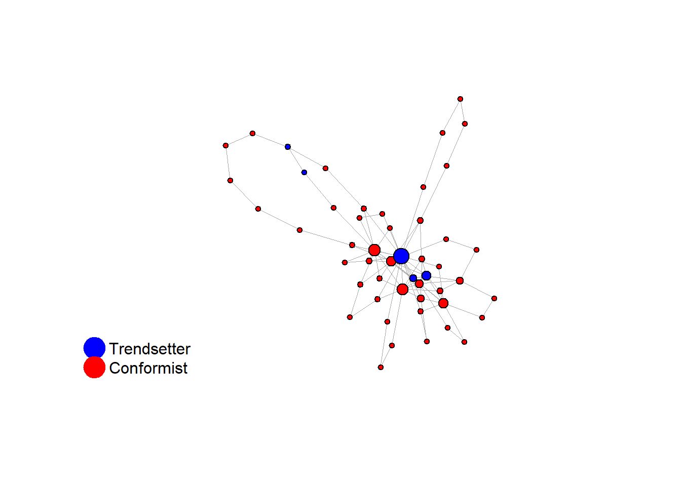
base = 2253281
seed = base + 2

# cbind(degree(test$network),V(test$network)$role)

# let's check the distribution of distances to 'trendsetters', among 'conformists'
g <- test$network
trend <- which(V(g)$role == "trendsetter")
conf <- which(V(g)$role == "conformist")

# distances: rows = sources (trendsetters), cols = all vertices
D <- distances(g, v = trend, to = V(g), mode = "all")
Dc <- D[, conf]  #keep just conformists

# calculate (a) the distance to the nearest trendsetter and (b) the average distance to
# trendsetters, across conformists
dists <- data.frame(shortest = apply(Dc, 2, min), average = apply(Dc, 2, function(x) mean(x[is.finite(x)])))
dists_long <- pivot_longer(dists, cols = c(shortest, average), names_to = "type", values_to = "distance_to_seed")

# plot the distribution
ggplot(dists_long, aes(x = distance_to_seed, fill = type)) + geom_histogram(bins = 20, alpha = 0.5, position = "identity") +
    theme_minimal()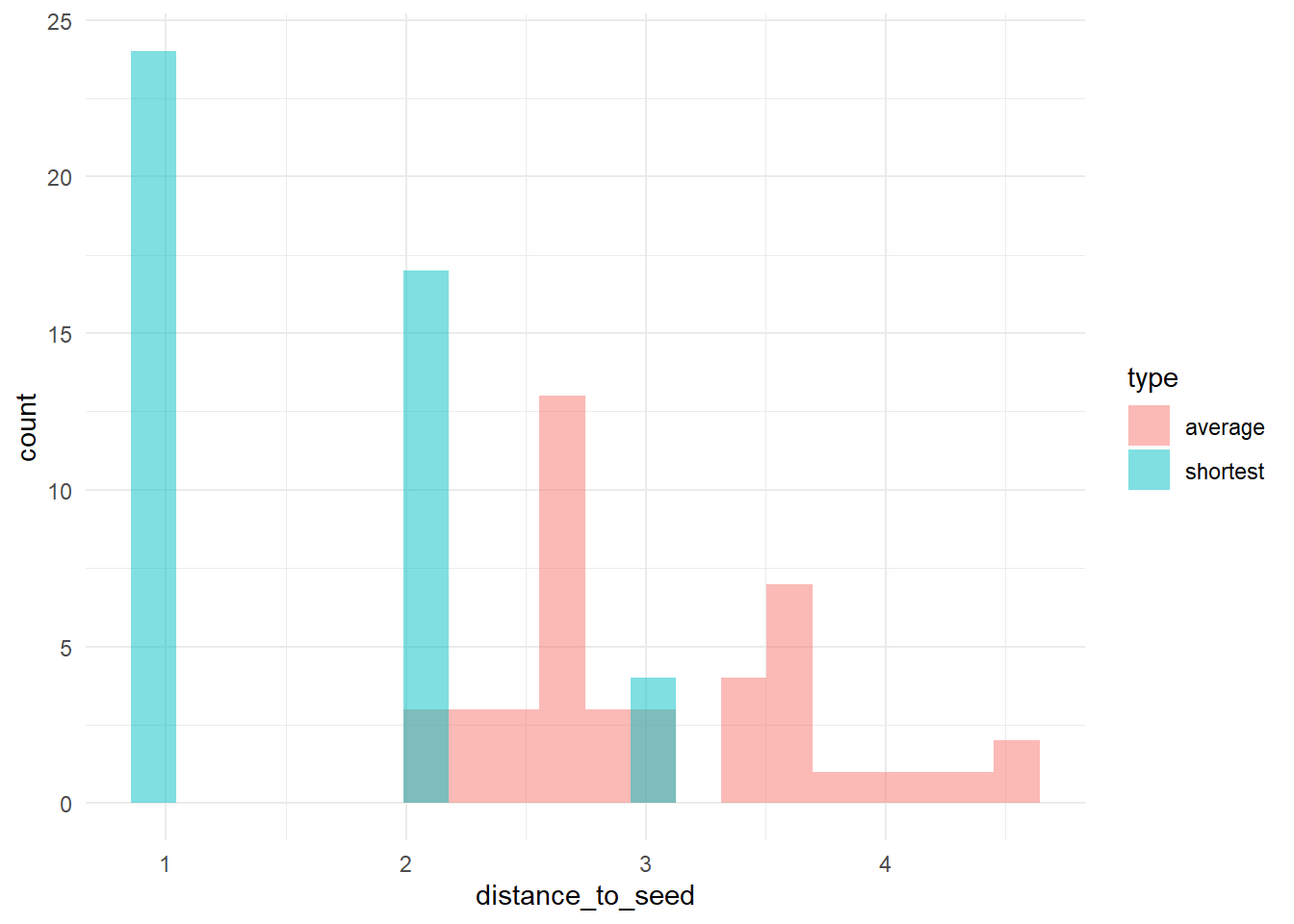
knitr::include_graphics(paste0("./figures/animation_network_", seed, ".gif"))
test <- run_one_seed(3, k_min = 2, k_max = 20, alpha = 2.4, rho = 0.4, r = -0.1)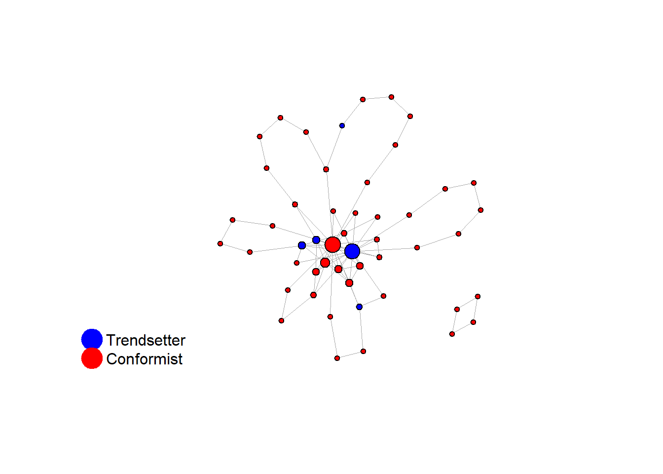
seed = seed + 1knitr::include_graphics(paste0("./figures/animation_network_", seed, ".gif"))
test <- run_one_seed(4, k_min = 2, k_max = 20, alpha = 2.4, rho = 0.4, r = -0.1, return_network = TRUE)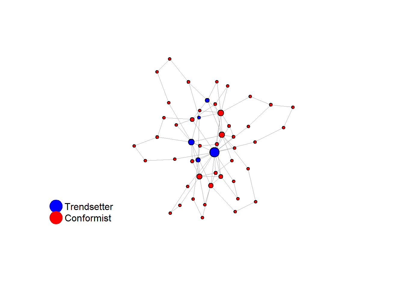
base = 2253281
seed = base + 4

# let's check the distribution of distances to 'trendsetters', among 'conformists'
g <- test$network
trend <- which(V(g)$role == "trendsetter")
conf <- which(V(g)$role == "conformist")

# distances: rows = sources (trendsetters), cols = all vertices
D <- distances(g, v = trend, to = V(g), mode = "all")
Dc <- D[, conf]  #keep just conformists

# calculate (a) the distance to the nearest trendsetter and (b) the average distance to
# trendsetters, across conformists
dists <- data.frame(shortest = apply(Dc, 2, min), average = apply(Dc, 2, function(x) mean(x[is.finite(x)])))
dists_long <- pivot_longer(dists, cols = c(shortest, average), names_to = "type", values_to = "distance_to_seed")

# plot the distribution
ggplot(dists_long, aes(x = distance_to_seed, fill = type)) + geom_histogram(bins = 20, alpha = 0.5, position = "identity") +
    theme_minimal()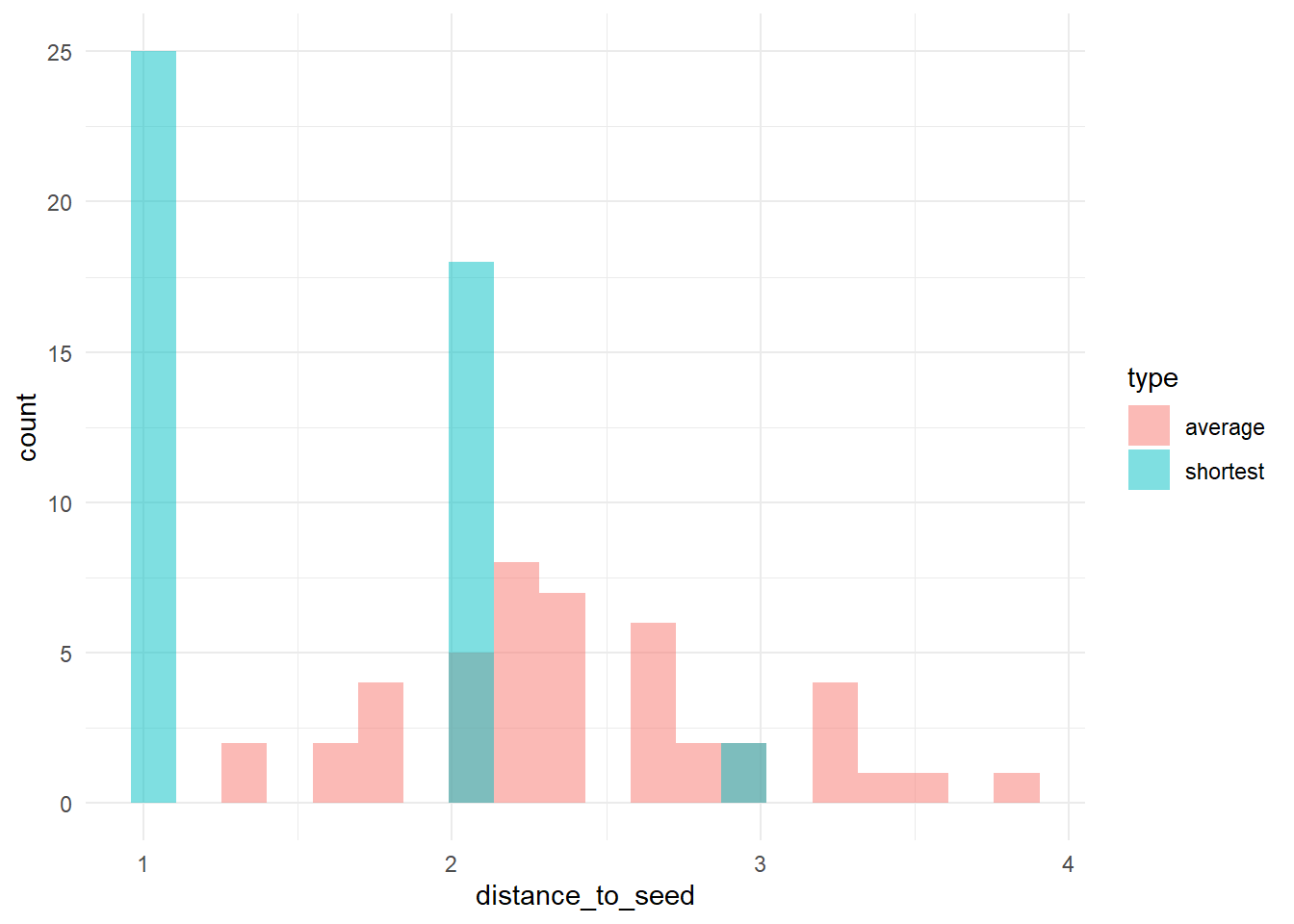
test$stats#> $run
#> [1] 4
#>
#> $seed
#> [1] 2253285
#>
#> $num_nodes
#> [1] 50
#>
#> $num_edges
#> [1] 89
#>
#> $avg_degree
#> [1] 3.56
#>
#> $sd_degree
#> [1] 3.091529
#>
#> $net_density
#> [1] 0.07265306
#>
#> $net_diameter
#> [1] 6
#>
#> $avg_path_len
#> [1] 2.923265
#>
#> $clust_coeff
#> [1] 0.1428571
#>
#> $assort_deg
#> [1] -0.09244437
#>
#> $deg_trait_cor
#> [1] 0.5489375
#>
#> $components
#> [1] 1table(degree(test$network))#>
#> 2 3 4 5 6 7 8 9 10 19
#> 29 8 3 3 1 1 1 1 2 1# identify trendsetters
ids <- which(V(test$network)$role == "trendsetter")
# check their centrality
sort(as.numeric(cbind(degree(test$network), V(test$network)$role)[ids]))#> [1] 3 5 6 10 19knitr::include_graphics(paste0("./figures/animation_network_", seed, ".gif"))
2.1.1 increased density
test <- run_one_seed(5, k_min = 2, k_max = 49, alpha = 2.4, rho = 0.4, r = -0.1, return_network = TRUE)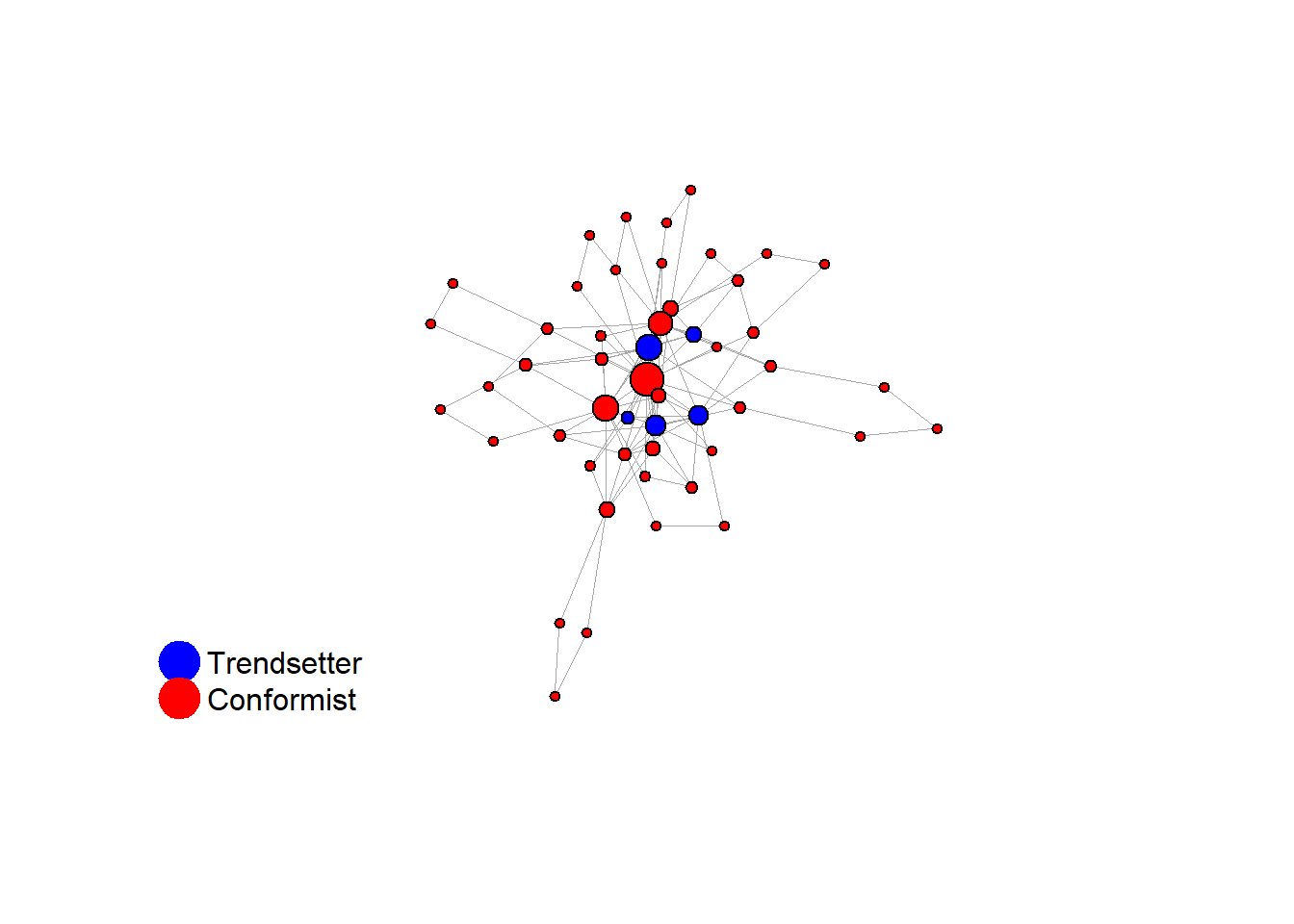
seed = seed + 1

# sort(degree(test$network)) cbind(degree(test$network), V(test$network)$role)

# let's check the distribution of distances to 'trendsetters', among 'conformists'
g <- test$network
trend <- which(V(g)$role == "trendsetter")
conf <- which(V(g)$role == "conformist")

# distances: rows = sources (trendsetters), cols = all vertices
D <- distances(g, v = trend, to = V(g), mode = "all")
Dc <- D[, conf]  #keep just conformists

# calculate (a) the distance to the nearest trendsetter and (b) the average distance to
# trendsetters, across conformists
dists <- data.frame(shortest = apply(Dc, 2, min), average = apply(Dc, 2, function(x) mean(x[is.finite(x)])))
dists_long <- pivot_longer(dists, cols = c(shortest, average), names_to = "type", values_to = "distance_to_seed")

# plot the distribution
ggplot(dists_long, aes(x = distance_to_seed, fill = type)) + geom_histogram(bins = 20, alpha = 0.5, position = "identity") +
    theme_minimal()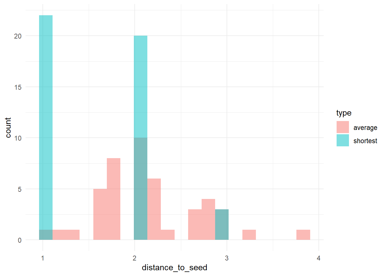
Let’s take this as our experimental network configuration.
test$stats#> $run
#> [1] 5
#>
#> $seed
#> [1] 2253286
#>
#> $num_nodes
#> [1] 50
#>
#> $num_edges
#> [1] 113
#>
#> $avg_degree
#> [1] 4.52
#>
#> $sd_degree
#> [1] 4.15142
#>
#> $net_density
#> [1] 0.0922449
#>
#> $net_diameter
#> [1] 6
#>
#> $avg_path_len
#> [1] 2.669388
#>
#> $clust_coeff
#> [1] 0.2378049
#>
#> $assort_deg
#> [1] -0.1081219
#>
#> $deg_trait_cor
#> [1] 0.4120337
#>
#> $components
#> [1] 1table(degree(test$network))#>
#> 2 3 4 5 6 7 10 11 14 15 21
#> 25 3 7 4 2 3 1 1 1 2 1# identify trendsetters
ids <- which(V(test$network)$role == "trendsetter")
# check their centrality
sort(as.numeric(cbind(degree(test$network), V(test$network)$role)[ids]))#> [1] 5 7 10 11 15# use this as the network structure for an otree session:
# cbind(degree(test$network),V(test$network)$role)
# convert to adjacency matrix
adj_matrix <- as.matrix(as_adjacency_matrix(test$network))
# get roles
role_vector <- ifelse(V(test$network)$role == "trendsetter", 1, 0)
# create a list to store the network data
net <- list(adj_matrix = adj_matrix, role_vector = role_vector)
# save the list as a JSON file
write_json(net, "network_test_n50.json")knitr::include_graphics(paste0("./figures/animation_network_", seed, ".gif"))
2.2 2. random network
with same number of ties
# ?erdos.renyi.game g <- erdos.renyi.game(n=50, p=0.05) ?sample_gnm()
set.seed(124124)
network <- sample_gnm(n = 50, m = 113)
V(network)$role <- sample(c(rep("trendsetter", 5), rep("conformist", 45)))

fplot_graph(network)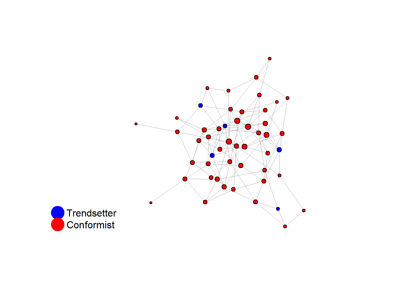
test <- fabm(network = network, max_rounds = 50, mi_threshold = 0.49, choice_rule = "probabilistic",
    plot = TRUE, histories = TRUE)

test$plot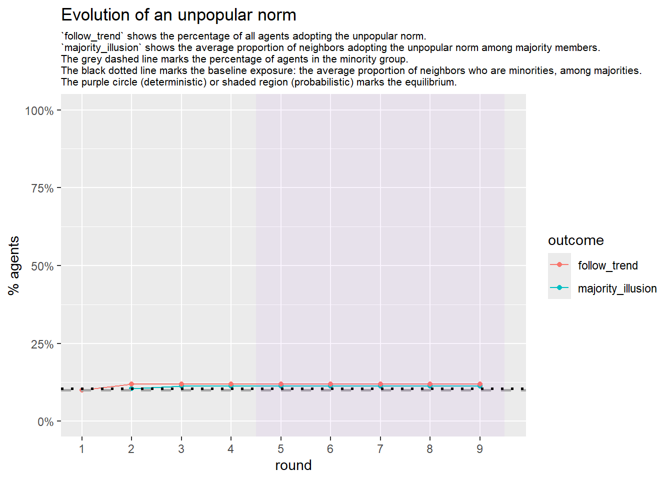
# let's check the distribution of distances to 'trendsetters', among 'conformists'
g <- network
trend <- which(V(g)$role == "trendsetter")
conf <- which(V(g)$role == "conformist")

# distances: rows = sources (trendsetters), cols = all vertices
D <- distances(g, v = trend, to = V(g), mode = "all")
Dc <- D[, conf]  #keep just conformists

# calculate (a) the distance to the nearest trendsetter and (b) the average distance to
# trendsetters, across conformists
dists <- data.frame(shortest = apply(Dc, 2, min), average = apply(Dc, 2, function(x) mean(x[is.finite(x)])))
dists_long <- pivot_longer(dists, cols = c(shortest, average), names_to = "type", values_to = "distance_to_seed")

# plot the distribution
ggplot(dists_long, aes(x = distance_to_seed, fill = type)) + geom_histogram(bins = 20, alpha = 0.5, position = "identity") +
    theme_minimal()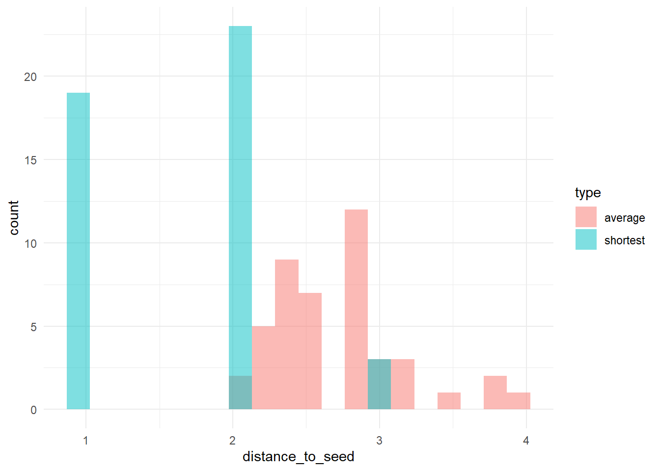
# --- stats ---
stats <- list(num_nodes = vcount(g), num_edges = ecount(g), avg_degree = mean(degree(g)), sd_degree = sd(degree(g)),
    net_density = edge_density(g), net_diameter = diameter(g, directed = FALSE, unconnected = TRUE),
    avg_path_len = average.path.length(g, directed = FALSE), clust_coeff = transitivity(g, type = "global"),
    assort_deg = assortativity_degree(g), deg_trait_cor = fdegtraitcor(g)$cor, components = components(g)$no)
stats
#> $num_nodes
#> [1] 50
#>
#> $num_edges
#> [1] 113
#>
#> $avg_degree
#> [1] 4.52
#>
#> $sd_degree
#> [1] 1.65665
#>
#> $net_density
#> [1] 0.0922449
#>
#> $net_diameter
#> [1] 5
#>
#> $avg_path_len
#> [1] 2.730612
#>
#> $clust_coeff
#> [1] 0.08387097
#>
#> $assort_deg
#> [1] 0.1327246
#>
#> $deg_trait_cor
#> [1] -0.02439024
#>
#> $components
#> [1] 1# use this as the network structure for an otree session:
# cbind(degree(test$network),V(test$network)$role)
# convert to adjacency matrix
adj_matrix <- as.matrix(as_adjacency_matrix(network))
# get roles
role_vector <- ifelse(V(network)$role == "trendsetter", 1, 0)
# create a list to store the network data
net <- list(adj_matrix = adj_matrix, role_vector = role_vector)
# save the list as a JSON file
write_json(net, "network_test_n50_random.json")3 import data
test <- read.csv("./rawdata/all_apps_wide_2026-02-02.csv")
times <- read.csv("./rawdata/PageTimes-2026-02-02.csv")
4 pilot results
On 2-2-2026, I recruited 80 Prolific participants, to populate a network of N=50 (with a 10% minority group):
4.1 arrival from Prolific
# subset experimental session
test <- test[test$session.code == "hwkqjhm0", ]
times <- times[times$session_code == "hwkqjhm0", ]

test <- test %>%
    transmute(participant_id = participant.code, participant_label = participant.label, id_in_session = participant.id_in_session,
        consent_given = consent.1.player.consent, consent_timestamp = consent.1.player.consent_timestamp,
        role = participant.role, is_dropout = participant.is_dropout, dropout_app = participant._current_app_name,
        comprehension_retries = comprehension.1.player.comprehension_retries, passed_comprehension = !participant._current_app_name %in%
            c("consent", "comprehension"), choice = unpop.1.player.choice)
test <- test[!is.na(test$consent_given), ]
test$bot <- ifelse(test$participant_label == "", 1, 0)

test <- test %>%
    mutate(consent_timestamp = ymd_hms(consent_timestamp), bot = factor(bot, levels = c(0, 1), labels = c("Prolific participant",
        "Bot"))) %>%
    arrange(consent_timestamp)

test <- test %>%
    mutate(arrival_order = row_number())

ggplot(test, aes(x = consent_timestamp, y = arrival_order)) + geom_point(aes(color = role, shape = bot),
    size = 3, alpha = 0.5) + scale_shape_manual(values = c(16, 2)) + scale_color_manual(values = c("blue",
    "red")) + labs(x = "Arrival time", y = "Arrival order", color = "Role", shape = "Type", title = "Participant arrivals from Prolific over time") +
    theme_minimal()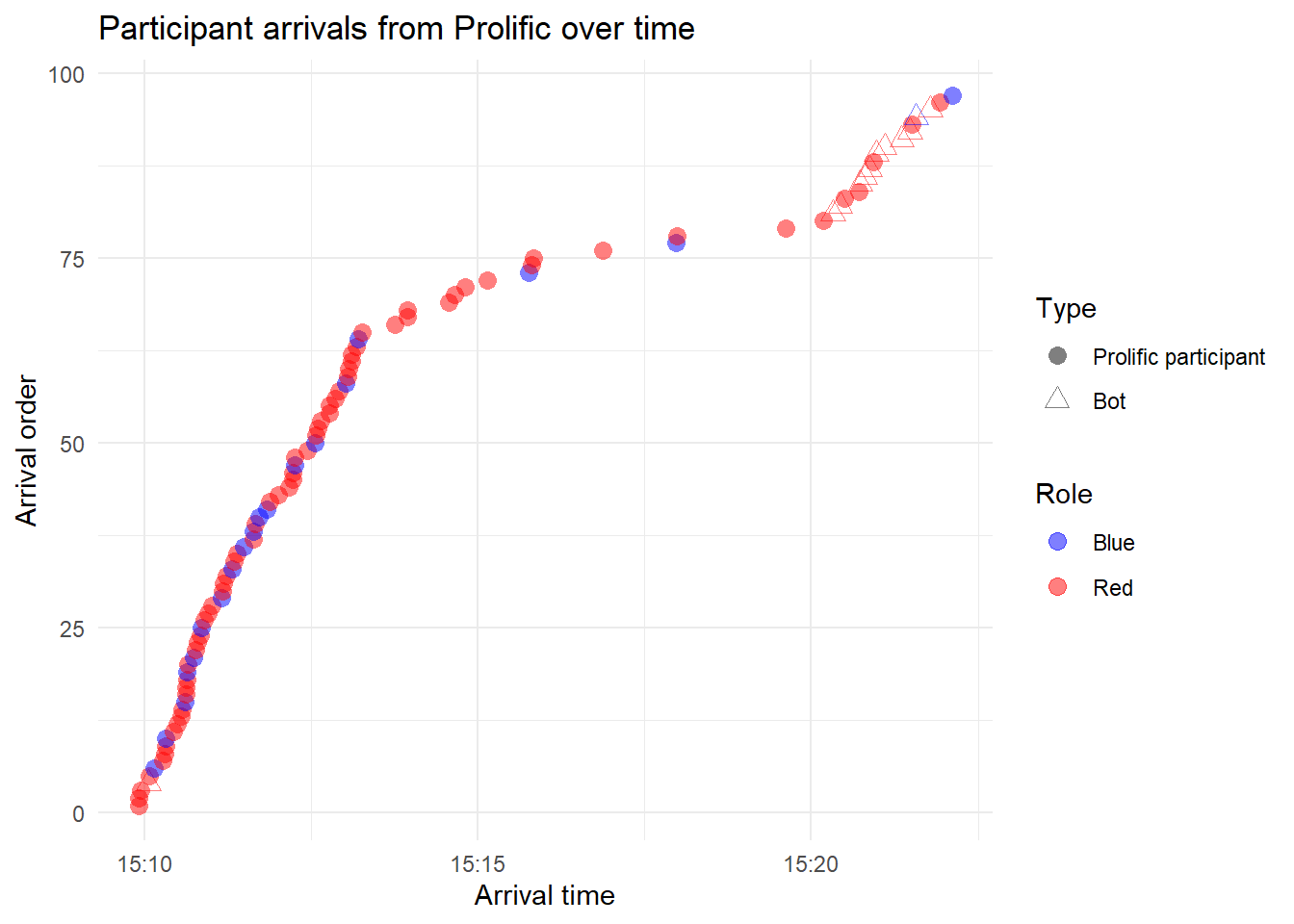
4.2 progression through the experiment
times <- times %>%
    mutate(timestamp = as_datetime(epoch_time_completed))

arrival_times <- times %>%
    group_by(participant_id_in_session) %>%
    summarize(arrival_time = min(timestamp), .groups = "drop")

times <- times %>%
    left_join(arrival_times, by = "participant_id_in_session") %>%
    mutate(participant_ordered = factor(participant_id_in_session, levels = arrival_times %>%
        arrange(arrival_time) %>%
        pull(participant_id_in_session)))

times_roles <- times %>%
    left_join(test %>%
        select(id_in_session, role), by = c(participant_id_in_session = "id_in_session"))

page_levels <- unique(times$page_name)

times_roles <- times_roles %>%
    mutate(page_name = factor(page_name, levels = page_levels))

custom_colors <- c(InitializeParticipant = "#c6dbef", ConsentPage = "#9ecae1", IntroductionPage = "#6baed6",
    ComprehensionPage = "#3182bd", NetworkFormationWaitPage = "#ffcc99", DecisionPage = "#ff9966", ResultsWaitPage = "#ff6666",
    ResultsPage = "#cc0033", FinalGameResults = "#660000")

# colored y-axis labels based on role
y_labels_colored <- times_roles %>%
    select(participant_ordered, role) %>%
    distinct() %>%
    arrange(participant_ordered) %>%
    mutate(label_colored = case_when(role == "Red" ~ paste0("<span style='color:red'>", participant_ordered,
        "</span>"), role == "Blue" ~ paste0("<span style='color:blue'>", participant_ordered, "</span>"),
        TRUE ~ paste0("<span style='color:darkgrey'>", participant_ordered, "</span>")))

# Create a named vector for scale_y_discrete labels
y_labels_vector <- y_labels_colored$label_colored
names(y_labels_vector) <- y_labels_colored$participant_ordered

# times2 <- times[times$participant_id_in_session %in% c(34,80),]

ggplot(times_roles, aes(x = timestamp, y = participant_ordered, color = page_name)) + geom_line(aes(group = participant_id_in_session),
    size = 1) + geom_point(size = 2) + scale_color_manual(values = custom_colors) + scale_y_discrete(labels = y_labels_vector) +
    labs(x = "Time", y = "Participant (ordered by arrival)", color = "Stage/Page", title = "Participant progression through experiment stages (by arrival)") +
    theme_minimal() + theme(axis.text.y = element_markdown(size = 6))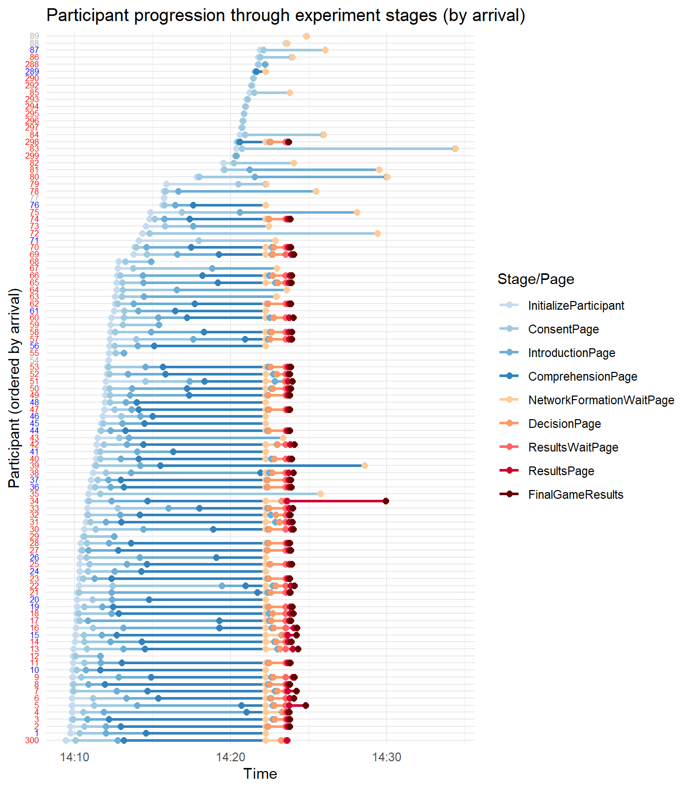
# by role
times_roles <- times %>%
    left_join(test %>%
        select(id_in_session, role), by = c(participant_id_in_session = "id_in_session"))

times_roles <- times_roles %>%
    mutate(page_name = factor(page_name, levels = page_levels))

colored_labels <- sapply(page_levels, function(stage) {
    paste0("<span style='color:", custom_colors[stage], "'>", stage, "</span>")
}, USE.NAMES = FALSE)

times_roles <- times_roles[!is.na(times_roles$role), ]

# Gantt-style plot faceted by participant role
ggplot(times_roles, aes(x = timestamp, y = page_name, group = participant_ordered, color = page_name)) +
    geom_step(direction = "hv", size = 0.5) + geom_point(size = 2) + scale_color_manual(values = custom_colors) +
    scale_y_discrete(labels = colored_labels) + labs(x = "Time", y = "Experiment Stage", color = "Stage/Page",
    title = "Participant progression through experiment stages by role") + facet_wrap(~role, scales = "free_y",
    ncol = 1) + theme_minimal() + theme(axis.text.y = element_markdown(size = 10), axis.text.x = element_text(angle = 45,
    hjust = 1), legend.position = "none")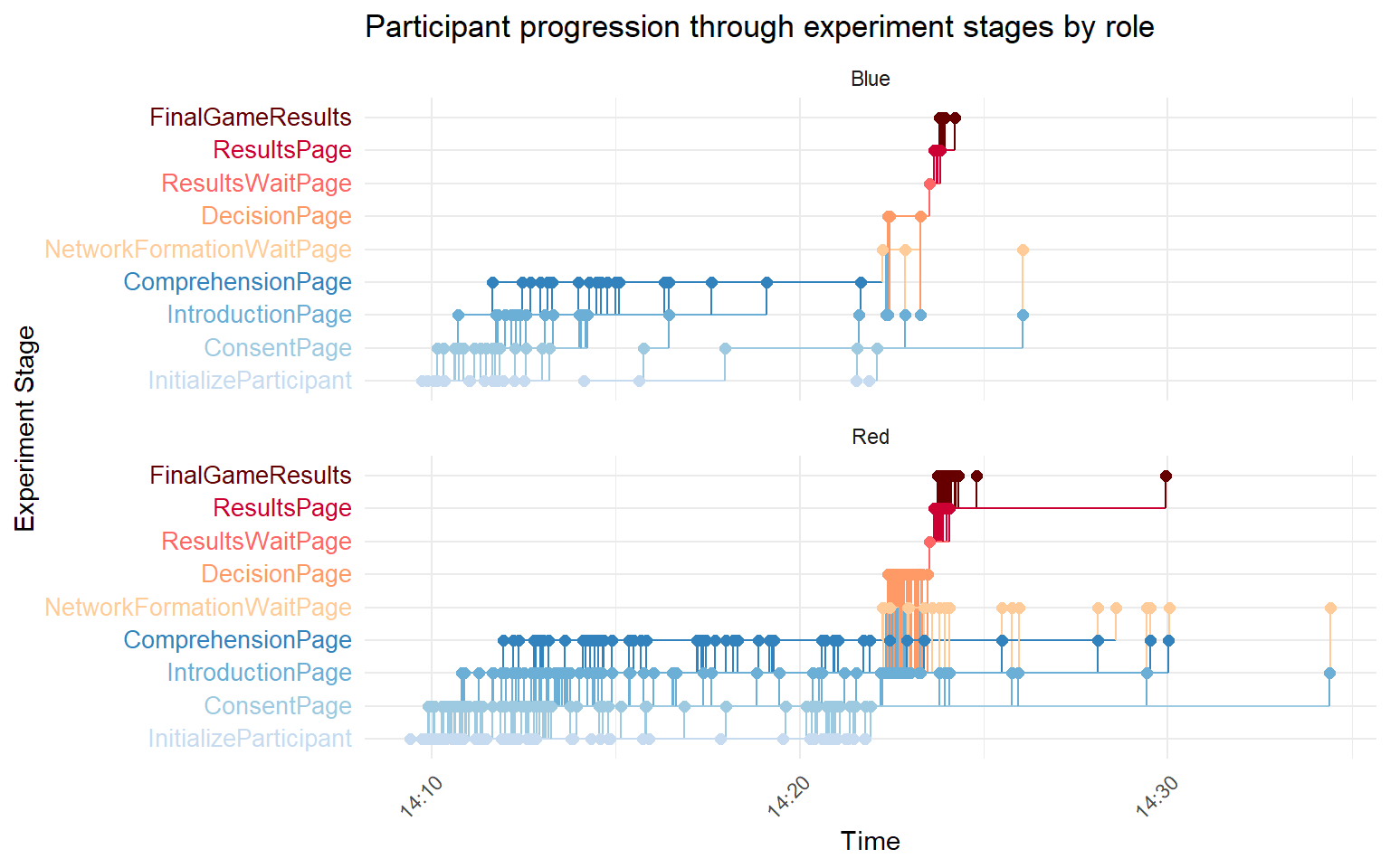
4.3 comprehension
Retries
table(test$comprehension_retries, test$role)#>
#> Blue Red
#> 0 5 38
#> 1 10 16
#> 2 3 8
#> 3 1 4
#> 4 1 3
#> 5 0 2
#> 7 0 1
#> 11 0 1
#> 12 0 1
#> 17 0 2
#> 21 0 1# time per comprehension task
times2 <- times %>%
filter(page_name == "ComprehensionPage") %>%
mutate(time_spent = as.numeric(timestamp - arrival_time))
# exclude bots
bots <- test$id_in_session[test$bot == "Bot"]
times3 <- times2[!times2$participant_id_in_session %in% bots, ]
comprehension_data <- times3 %>%
left_join(test %>%
select(id_in_session, comprehension_retries, role), by = c(participant_id_in_session = "id_in_session"))
ggplot(comprehension_data, aes(x = time_spent, y = factor(comprehension_retries), color = role)) + geom_jitter(width = 0,
height = 0.2, size = 2, alpha = 0.7) + scale_color_manual(values = c("blue", "red")) + labs(x = "Time spent on comprehension (seconds)",
y = "Number of retries", color = "Role", title = "Time in seconds") + theme_minimal(base_size = 14)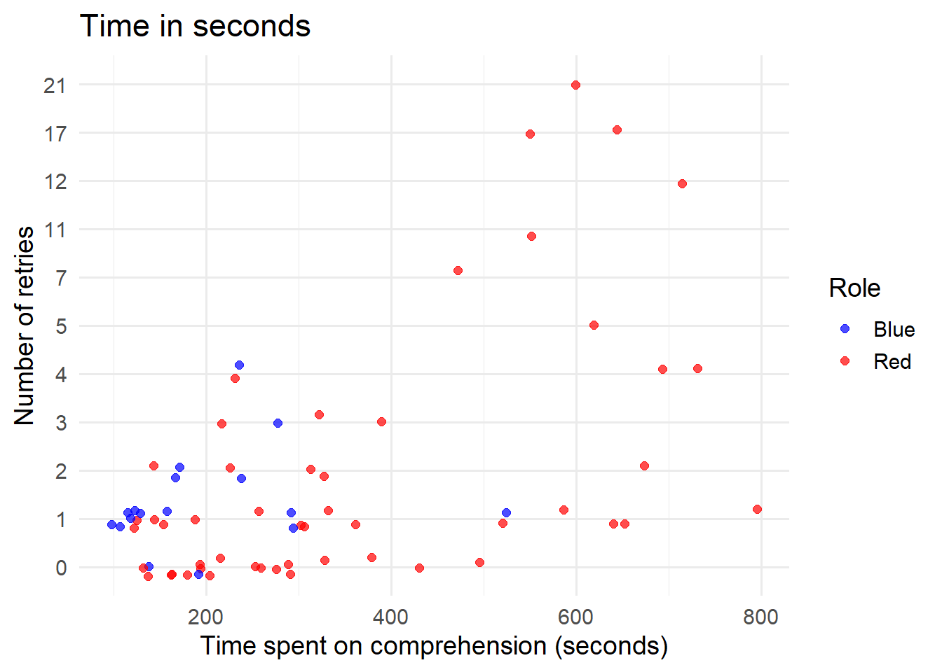
4.4 choice behavior
# exclude bots and missing choices
test2 <- test %>%
    filter(bot != "Bot") %>%
    select(id_in_session, role, choice, comprehension_retries) %>%
    filter(!is.na(choice))

# scatter plot: choice vs role, size = retries
ggplot(test2, aes(x = role, y = as.numeric(choice), size = comprehension_retries)) + geom_jitter(width = 0.2,
    height = 0.05, alpha = 0.7, color = "steelblue") + scale_size_continuous(range = c(2, 8)) + labs(x = "Participant role",
    y = "Choice (1=blue, 0=red)", size = "Number of retries", title = "Participant choice by role and comprehension question retries") +
    theme_minimal(base_size = 14)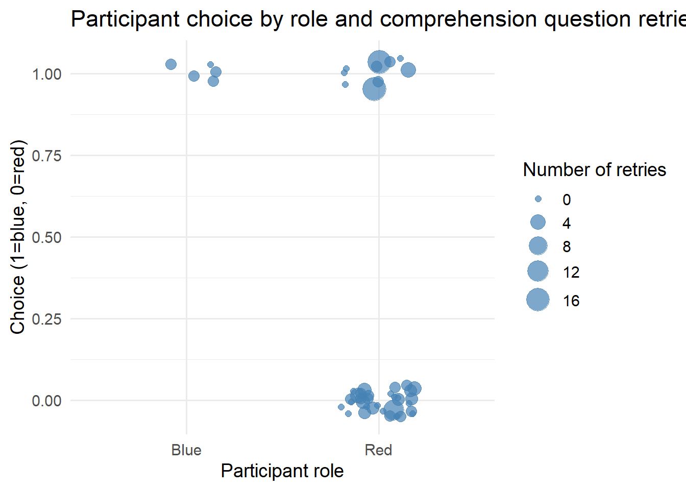
LS0tDQp0aXRsZTogIkV4cGVyaW1lbnQiDQpiaWJsaW9ncmFwaHk6IHJlZmVyZW5jZXMuYmliDQpsaW5rLWNpdGF0aW9uczogdHJ1ZQ0KZGF0ZTogIkxhc3QgY29tcGlsZWQgb24gYHIgZm9ybWF0KFN5cy50aW1lKCksICclZC0lbS0lWScpYCINCm91dHB1dDogDQogIGh0bWxfZG9jdW1lbnQ6DQogICAgc2VsZl9jb250YWluZWQ6IHRydWUNCiAgICBjc3M6IHR3ZWFrcy5jc3MNCiAgICB0b2M6IHRydWUNCiAgICB0b2NfZmxvYXQ6IHRydWUNCiAgICBudW1iZXJfc2VjdGlvbnM6IHRydWUNCiAgICB0b2NfZGVwdGg6IDQNCiAgICBjb2RlX2ZvbGRpbmc6IHNob3cNCiAgICBjb2RlX2Rvd25sb2FkOiB5ZXMNCi0tLQ0KDQpgYGB7ciwgZ2xvYmFsc2V0dGluZ3MsIGVjaG89RkFMU0UsIHdhcm5pbmc9RkFMU0UsIHJlc3VsdHM9J2hpZGUnLCBtZXNzYWdlPUZBTFNFfQ0KbGlicmFyeShrbml0cikNCmxpYnJhcnkodGlkeXZlcnNlKQ0Ka25pdHI6Om9wdHNfY2h1bmskc2V0KGVjaG8gPSBUUlVFKQ0Kb3B0c19jaHVuayRzZXQodGlkeS5vcHRzPWxpc3Qod2lkdGguY3V0b2ZmPTEwMCksdGlkeT1UUlVFLCB3YXJuaW5nID0gRkFMU0UsIG1lc3NhZ2UgPSBGQUxTRSxjb21tZW50ID0gIiM+IiwgY2FjaGU9VFJVRSwgY2xhc3Muc291cmNlPWMoInRlc3QiKSwgY2xhc3Mub3V0cHV0PWMoInRlc3QzIikpDQpvcHRpb25zKHdpZHRoID0gMTAwKQ0KcmdsOjpzZXR1cEtuaXRyKCkNCg0KY29sb3JpemUgPC0gZnVuY3Rpb24oeCwgY29sb3IpIHtzcHJpbnRmKCI8c3BhbiBzdHlsZT0nY29sb3I6ICVzOyc+JXM8L3NwYW4+IiwgY29sb3IsIHgpIH0NCmBgYA0KDQpgYGB7ciBrbGlwcHksIGVjaG89RkFMU0UsIGluY2x1ZGU9VFJVRX0NCmtsaXBweTo6a2xpcHB5KHBvc2l0aW9uID0gYygndG9wJywgJ3JpZ2h0JykpDQoja2xpcHB5OjprbGlwcHkoY29sb3IgPSAnZGFya3JlZCcpDQoja2xpcHB5OjprbGlwcHkodG9vbHRpcF9tZXNzYWdlID0gJ0NsaWNrIHRvIGNvcHknLCB0b29sdGlwX3N1Y2Nlc3MgPSAnRG9uZScpDQpgYGANCg0KLS0tDQoNCiMgR2V0dGluZyBzdGFydGVkDQoNClRvIGNvcHkgdGhlIGNvZGUsIGNsaWNrIHRoZSBidXR0b24gaW4gdGhlIHVwcGVyIHJpZ2h0IGNvcm5lciBvZiB0aGUgY29kZS1jaHVua3MuDQoNCiMjIGNsZWFuIHVwDQoNCmBgYHtyLCBjbGVhbl91cCwgcmVzdWx0cz0naGlkZSd9DQpybShsaXN0PWxzKCkpDQpnYygpDQpgYGANCg0KPGJyPg0KDQojIyBjdXN0b20gZnVuY3Rpb25zDQoNCldlIGRlZmluZWQgYSBudW1iZXIgY3VzdG9tIGZ1bmN0aW9ucywgYXQgYHIgeGZ1bjo6ZW1iZWRfZmlsZSgiLi9jdXN0b21fZnVuY3Rpb25zLlIiKWAuDQoNCmBgYHtyLCBjdXN0b21fZnVuY3Rpb25zfQ0Kc291cmNlKCIuL2N1c3RvbV9mdW5jdGlvbnMuUiIpDQpgYGANCg0KPGJyPg0KDQojIyBuZWNlc3NhcnkgcGFja2FnZXMNCg0KLSBgdGlkeXZlcnNlYDogZGF0YSB3cmFuZ2xpbmcNCi0gYGlncmFwaGA6IGdlbmVyYXRlIGFuZCB2aXN1YWxpemUgZ3JhcGhzDQotIGBwYXJhbGxlbGA6IHBhcmFsbGVsIGNvbXB1dGluZyB0byBzcGVlZCB1cCBzaW11bGF0aW9uDQotIGBmb3JlYWNoYDogbG9vcGluZyBpbiBwYXJhbGxlbA0KLSBgZG9QYXJhbGxlbGA6IHBhcmFsbGVsIGJhY2tlbmQgZm9yIGBmb3JlYWNoYA0KLSBgZ2dwbG90MmA6IGRhdGEgdmlzdWFsaXphdGlvbg0KLSBgZ2doNHhgOiBoYWNrcyBmb3IgYGdncGxvdDJgDQotIGBnZ3B1YnJgOiBtYWtlIHZpc3VhbGl6YXRpb25zIHB1YmxpY2F0aW9uLXJlYWR5DQoNCmBgYHtyLCBwYWNrYWdlc30NCnBhY2thZ2VzID0gYygidGlkeXZlcnNlIiwgImlncmFwaCIsICJnZ3Bsb3QyIiwgInBhcmFsbGVsIiwgImRvUGFyYWxsZWwiLCAiZm9yZWFjaCIsICJnZ2g0eCIsICJnZ3B1YnIiLCAicGxvdGx5IiwgIlJDb2xvckJyZXdlciIsICJncmlkIiwgImdyaWRFeHRyYSIsICJwYXRjaHdvcmsiLCAiZ2dwbG90aWZ5IiwgImdncmFwaCIsICJnZ2FuaW1hdGUiLCAiUkNvbG9yQnJld2VyIiwNCiAgICAiZ2d0ZXh0IiwgIm1hZ2ljayIsICJqc29ubGl0ZSIsICJsdWJyaWRhdGUiLCAiZ2d0ZXh0IikNCg0KaW52aXNpYmxlKGZwYWNrYWdlLmNoZWNrKHBhY2thZ2VzKSkNCnJtKHBhY2thZ2VzKQ0KYGBgDQoNCi0tLQ0KDQojIEV4cGVyaW1lbnRhbCBjb25kaXRpb25zDQoNCiMjIDEuIGhlYXZ5LXRhaWxlZCBuZXR3b3JrIHdpdGggY2VudHJhbCBtaW5vcml0aWVzDQoNCkxldCdzIHRha2UgYSBsaWtlbHktY2FzZSBmb3IgYW4gdW5wb3B1bGFyIG5vcm0sIGdlbmVyYXRlIG11bHRpcGxlIG5ldHdvcmtzIG9mIHRoaXMgdGFyZ2V0LCBhbmQgc2ltdWxhdGUgdGhlIGVtZXJnZW5jZSBvZiB0aGUgbm9ybSBmb2xsb3dpbmcgYSBkZXRlcm1pbmlzdGljIGFuZCBwcm9iYWJpbGlzdGljIGNob2ljZSBtb2RlbDoNCg0KYGBge3IsIGVjaG89VFJVRSwgZmlnLnNob3c9J2hvbGQnLCBmaWcua2VlcD0nYWxsJywgbWVzc2FnZT1GQUxTRSwgZmlnLmhlaWdodD01fQ0KIyBwaWNrIG9uZSBjb25maWd1cmF0aW9uIHRoYXQgbGlrZWx5IGxlYWRzIHRvIGFuIHVucG9wdWxhciBub3JtLCBhbmQgZXhwbG9yZSBtdWx0aXBsZSAnc2VlZHMnOg0KcnVuX29uZV9zZWVkIDwtIGZ1bmN0aW9uKA0KICBpLA0KICBiYXNlX3NlZWQgPSAyMjUzMjgxLA0KICBwYXJhbXMgPSBsaXN0KHMgPSAxNSwgZSA9IDEwLCB3ID0gNDAsIHogPSA1MCwgbGFtYmRhMSA9IDUsIGxhbWJkYTIgPSAxLjgpLA0KICANCiAgIyB0d2VhayBuZXR3b3JrDQogIGtfbWluID0gMiwgDQogIGtfbWF4ID0gMjAsDQogIGFscGhhID0gMi40LA0KICByaG8gPSAwLjQsDQogIHIgPSAtMC4xLA0KICANCiAgIyByZXRyaWV2ZSBuZXR3b3JrDQogIHJldHVybl9uZXR3b3JrID0gRkFMU0UNCiAgDQopIHsNCiAgIyBkZXJpdmVkIHNlZWQgZm9yIHRoaXMgcnVuDQogIHNlZWRfaSA8LSBiYXNlX3NlZWQgKyBpDQogIHNldC5zZWVkKHNlZWRfaSkNCg0KICAjIC0tLSBuZXR3b3JrIGNyZWF0aW9uIC0tLQ0KICBkZWdzZXEgPC0gZmRlZ3NlcSgNCiAgICBuICAgICAgPSA1MCwNCiAgICBhbHBoYSAgPSBhbHBoYSwNCiAgICBrX21pbiAgPSBrX21pbiwNCiAgICBrX21heCAgPSBrX21heCwNCiAgICBkaXN0ICAgPSAibG9nLW5vcm1hbCIsICN1c2UgbG9nLW5vcm1hbCANCiAgICBzZWVkICAgPSBzZWVkX2kNCiAgKQ0KDQogIG5ldHdvcmsgPC0gc2FtcGxlX2RlZ3NlcShkZWdzZXEsIG1ldGhvZCA9ICJ2bCIpDQogIA0KICBWKG5ldHdvcmspJHJvbGUgPC0gc2FtcGxlKA0KICAgIGMocmVwKCJ0cmVuZHNldHRlciIsIDUpLCByZXAoImNvbmZvcm1pc3QiLCA0NSkpDQogICkNCiAgDQoNCiAgcmV3aXJlZF9uZXR3b3JrIDwtIGZyZXdpcmVfcihuZXR3b3JrLCByLCB2ZXJib3NlID0gRkFMU0UsIG1heF9pdGVyID0gMWU1KQ0KICBmaW5hbF9uZXR3b3JrICAgPC0gZnN3YXBfcmhvKHJld2lyZWRfbmV0d29yaywgcmhvLCB2ZXJib3NlID0gRkFMU0UsIG1heF9pdGVyID0gMWU0KQ0KICANCiAgIyAtLS0gc3RhdHMgLS0tDQogIHN0YXRzIDwtIGxpc3QoDQogICAgcnVuICAgICAgICAgICA9IGksDQogICAgc2VlZCAgICAgICAgICA9IHNlZWRfaSwNCiAgICBudW1fbm9kZXMgICAgID0gdmNvdW50KGZpbmFsX25ldHdvcmspLA0KICAgIG51bV9lZGdlcyAgICAgPSBlY291bnQoZmluYWxfbmV0d29yayksDQogICAgYXZnX2RlZ3JlZSAgICA9IG1lYW4oZGVncmVlKGZpbmFsX25ldHdvcmspKSwNCiAgICBzZF9kZWdyZWUgICAgID0gc2QoZGVncmVlKGZpbmFsX25ldHdvcmspKSwNCiAgICBuZXRfZGVuc2l0eSAgID0gZWRnZV9kZW5zaXR5KGZpbmFsX25ldHdvcmspLA0KICAgIG5ldF9kaWFtZXRlciAgPSBkaWFtZXRlcihmaW5hbF9uZXR3b3JrLCBkaXJlY3RlZCA9IEZBTFNFLCB1bmNvbm5lY3RlZCA9IFRSVUUpLA0KICAgIGF2Z19wYXRoX2xlbiAgPSBhdmVyYWdlLnBhdGgubGVuZ3RoKGZpbmFsX25ldHdvcmssIGRpcmVjdGVkID0gRkFMU0UpLA0KICAgIGNsdXN0X2NvZWZmICAgPSB0cmFuc2l0aXZpdHkoZmluYWxfbmV0d29yaywgdHlwZSA9ICJnbG9iYWwiKSwNCiAgICBhc3NvcnRfZGVnICAgID0gYXNzb3J0YXRpdml0eV9kZWdyZWUoZmluYWxfbmV0d29yayksDQogICAgZGVnX3RyYWl0X2NvciA9IGZkZWd0cmFpdGNvcihmaW5hbF9uZXR3b3JrKSRjb3IsDQogICAgY29tcG9uZW50cyAgICA9IGNvbXBvbmVudHMoZmluYWxfbmV0d29yaykkbm8NCiAgKQ0KICANCiAgZnBsb3RfZ3JhcGgoZmluYWxfbmV0d29yaywgbGF5b3V0ID0gbGF5b3V0X3dpdGhfZnIoZmluYWxfbmV0d29yaykpIA0KICANCiAgDQogICMgLS0tIGluaXRpYWwgYWN0aW9ucyAtLS0NCiAgVihmaW5hbF9uZXR3b3JrKSRhY3Rpb24gPC0gaWZlbHNlKFYoZmluYWxfbmV0d29yaykkcm9sZSA9PSAidHJlbmRzZXR0ZXIiLCAxLCAwKQ0KICANCiAgIyAtLS0gZGV0ZXJtaW5pc3RpYyBzaW11bGF0aW9uIC0tLQ0KICBzaW1fZGV0IDwtIGZhYm0oDQogICAgbmV0d29yayAgICAgID0gZmluYWxfbmV0d29yaywNCiAgICBwYXJhbXMgICAgICAgPSBwYXJhbXMsDQogICAgbWF4X3JvdW5kcyAgID0gNTAsDQogICAgbWlfdGhyZXNob2xkID0gMC40OSwNCiAgICBjaG9pY2VfcnVsZSAgPSAiZGV0ZXJtaW5pc3RpYyIsDQogICAgcGxvdCAgICAgICAgID0gVFJVRSwNCiAgICBoaXN0b3JpZXMgICAgPSBUUlVFDQogICkNCiAgDQogICMgZ2VuZXJhdGUgdGhlIGdpZiBmb3IgdGhlIGN1cnJlbnQgbmV0d29yaw0KICBnaWZfZmlsZW5hbWUgPC0gcGFzdGUwKCIuL2ZpZ3VyZXMvYW5pbWF0aW9uX25ldHdvcmtfIiwgc2VlZF9pLCAiLmdpZiIpDQogIGdpZl9wYXRoIDwtIGZuZXR3b3JrZ2lmKGZpbmFsX25ldHdvcmssIHNpbV9kZXQkZGVjaXNpb25faGlzdG9yeSwgcm91bmRzID0gc2ltX2RldCRlcXVpbGlicml1bSRyb3VuZCwgb3V0cHV0X2RpciA9ICIuL2ZpZ3VyZXMiKQ0KICAjIHJlbmFtZSB0aGUgZ2lmIHRvIG1hdGNoIHRoZSBuYW1pbmcgcGF0dGVybg0KICBmaWxlLnJlbmFtZShnaWZfcGF0aCwgZ2lmX2ZpbGVuYW1lKQ0KDQogIGlmICghaXMubnVsbChzaW1fZGV0JHBsb3QpKSB7DQogICAgcHJpbnQoc2ltX2RldCRwbG90KQ0KICB9DQogIA0KICAjIC0tLSBwcm9iYWJpbGlzdGljIHNpbXVsYXRpb24gLS0tDQogIHNpbV9wcm9iIDwtIGZhYm0oDQogICAgbmV0d29yayAgICAgICAgICAgICAgICA9IGZpbmFsX25ldHdvcmssDQogICAgcGFyYW1zICAgICAgICAgICAgICAgICA9IHBhcmFtcywNCiAgICBtYXhfcm91bmRzICAgICAgICAgICAgID0gMTAwLA0KICAgIG1pX3RocmVzaG9sZCAgICAgICAgICAgPSAwLjQ5LA0KICAgIGNob2ljZV9ydWxlICAgICAgICAgICAgPSAicHJvYmFiaWxpc3RpYyIsDQogICAgc3RhYmxlX3dpbmRvdyAgICAgICAgICA9IDgsICAgIyB0aGUgbGVuZ3RoIG9mIHRoZSB3aW5kb3cgb2YgYWRvcHRpb24gdmFsdWVzDQogICAgcmVxdWlyZWRfc3RhYmxlX3JvdW5kcyA9IDIwLCAjIG51bWJlciBvZiB3aW5kb3dzIG5lZWRlZCB0byBkZWNsYXJlIGVxdWlsaWJyaXVtDQogICAgcGxvdCAgICAgICAgICAgICAgICAgICA9IFRSVUUNCiAgKQ0KICBpZiAoIWlzLm51bGwoc2ltX3Byb2IkcGxvdCkpIHsNCiAgICBwcmludChzaW1fcHJvYiRwbG90KQ0KICB9DQogIA0KICAgcmVzdWx0IDwtIGxpc3QoDQogICAgc2VncmVnYXRpb25fZGV0ICA9IHNpbV9kZXQkZXF1aWxpYnJpdW0kc2VncmVnYXRpb24sDQogICAgc2VncmVnYXRpb25fcHJvYiA9IHNpbV9wcm9iJGVxdWlsaWJyaXVtJHNlZ3JlZ2F0aW9uLA0KICAgIHN0YXRzICAgICAgICAgICAgPSBzdGF0cw0KICApDQogIA0KICBpZiAocmV0dXJuX25ldHdvcmspIHsNCiAgICByZXN1bHQkbmV0d29yayA8LSBmaW5hbF9uZXR3b3JrDQogIH0NCiAgDQogIHJlc3VsdA0KfQ0KDQpgYGANCg0KDQpgYGB7cn0NCnRlc3QgPC0gcnVuX29uZV9zZWVkKDIsIGtfbWluID0gMiwga19tYXggPSAyMCwgYWxwaGEgPSAyLjQsIHJobyA9IDAuNCwgciA9IC0wLjEsIHJldHVybl9uZXR3b3JrID0gVFJVRSkNCg0KYmFzZSA9IDIyNTMyODENCnNlZWQgPSBiYXNlICsgMg0KDQojY2JpbmQoZGVncmVlKHRlc3QkbmV0d29yayksVih0ZXN0JG5ldHdvcmspJHJvbGUpDQoNCiNsZXQncyBjaGVjayB0aGUgZGlzdHJpYnV0aW9uIG9mIGRpc3RhbmNlcyB0byAndHJlbmRzZXR0ZXJzJywgYW1vbmcgJ2NvbmZvcm1pc3RzJw0KZyA8LSB0ZXN0JG5ldHdvcmsNCnRyZW5kIDwtIHdoaWNoKFYoZykkcm9sZSA9PSAidHJlbmRzZXR0ZXIiKQ0KY29uZiAgPC0gd2hpY2goVihnKSRyb2xlID09ICJjb25mb3JtaXN0IikNCg0KIyBkaXN0YW5jZXM6IHJvd3MgPSBzb3VyY2VzICh0cmVuZHNldHRlcnMpLCBjb2xzID0gYWxsIHZlcnRpY2VzDQpEIDwtIGRpc3RhbmNlcyhnLCB2ID0gdHJlbmQsIHRvID0gVihnKSwgbW9kZSA9ICJhbGwiKQ0KRGMgPC0gRFssIGNvbmZdICNrZWVwIGp1c3QgY29uZm9ybWlzdHMNCg0KIyBjYWxjdWxhdGUgKGEpIHRoZSBkaXN0YW5jZSB0byB0aGUgbmVhcmVzdCB0cmVuZHNldHRlciBhbmQgKGIpIHRoZSBhdmVyYWdlIGRpc3RhbmNlIHRvIHRyZW5kc2V0dGVycywgYWNyb3NzIGNvbmZvcm1pc3RzDQpkaXN0cyA8LSBkYXRhLmZyYW1lKA0KICBzaG9ydGVzdCA9IGFwcGx5KERjLCAyLCBtaW4pLA0KICBhdmVyYWdlID0gYXBwbHkoRGMsIDIsIGZ1bmN0aW9uKHgpIG1lYW4oeFtpcy5maW5pdGUoeCldKSkNCikNCmRpc3RzX2xvbmcgPC0gcGl2b3RfbG9uZ2VyKA0KICBkaXN0cywNCiAgY29scyA9IGMoc2hvcnRlc3QsIGF2ZXJhZ2UpLA0KICBuYW1lc190byA9ICJ0eXBlIiwNCiAgdmFsdWVzX3RvID0gImRpc3RhbmNlX3RvX3NlZWQiDQopDQoNCiNwbG90IHRoZSBkaXN0cmlidXRpb24NCmdncGxvdChkaXN0c19sb25nLCBhZXMoeCA9IGRpc3RhbmNlX3RvX3NlZWQsIGZpbGwgPSB0eXBlKSkgKw0KICBnZW9tX2hpc3RvZ3JhbSgNCiAgICBiaW5zID0gMjAsDQogICAgYWxwaGEgPSAwLjUsDQogICAgcG9zaXRpb24gPSAiaWRlbnRpdHkiDQogICkgKw0KICB0aGVtZV9taW5pbWFsKCkNCmBgYA0KDQoNCmBgYHtyLCBvdXQud2lkdGg9IjYwJSJ9DQprbml0cjo6aW5jbHVkZV9ncmFwaGljcyhwYXN0ZTAoIi4vZmlndXJlcy9hbmltYXRpb25fbmV0d29ya18iLCBzZWVkICwiLmdpZiIpKQ0KYGBgDQoNCmBgYHtyfQ0KdGVzdCA8LSBydW5fb25lX3NlZWQoMywga19taW4gPSAyLCBrX21heCA9IDIwLCBhbHBoYSA9IDIuNCwgcmhvID0gMC40LCByID0gLTAuMSkNCnNlZWQgPSBzZWVkICsgMQ0KYGBgDQoNCmBgYHtyLCBvdXQud2lkdGg9IjYwJSJ9DQprbml0cjo6aW5jbHVkZV9ncmFwaGljcyhwYXN0ZTAoIi4vZmlndXJlcy9hbmltYXRpb25fbmV0d29ya18iLCBzZWVkICwiLmdpZiIpKQ0KYGBgDQoNCmBgYHtyfQ0KdGVzdCA8LSBydW5fb25lX3NlZWQoNCwga19taW4gPSAyLCBrX21heCA9IDIwLCBhbHBoYSA9IDIuNCwgcmhvID0gMC40LCByID0gLTAuMSwgcmV0dXJuX25ldHdvcmsgPSBUUlVFKQ0KYmFzZSA9IDIyNTMyODENCnNlZWQgPSBiYXNlICsgNA0KDQojbGV0J3MgY2hlY2sgdGhlIGRpc3RyaWJ1dGlvbiBvZiBkaXN0YW5jZXMgdG8gJ3RyZW5kc2V0dGVycycsIGFtb25nICdjb25mb3JtaXN0cycNCmcgPC0gdGVzdCRuZXR3b3JrDQp0cmVuZCA8LSB3aGljaChWKGcpJHJvbGUgPT0gInRyZW5kc2V0dGVyIikNCmNvbmYgIDwtIHdoaWNoKFYoZykkcm9sZSA9PSAiY29uZm9ybWlzdCIpDQoNCiMgZGlzdGFuY2VzOiByb3dzID0gc291cmNlcyAodHJlbmRzZXR0ZXJzKSwgY29scyA9IGFsbCB2ZXJ0aWNlcw0KRCA8LSBkaXN0YW5jZXMoZywgdiA9IHRyZW5kLCB0byA9IFYoZyksIG1vZGUgPSAiYWxsIikNCkRjIDwtIERbLCBjb25mXSAja2VlcCBqdXN0IGNvbmZvcm1pc3RzDQoNCiMgY2FsY3VsYXRlIChhKSB0aGUgZGlzdGFuY2UgdG8gdGhlIG5lYXJlc3QgdHJlbmRzZXR0ZXIgYW5kIChiKSB0aGUgYXZlcmFnZSBkaXN0YW5jZSB0byB0cmVuZHNldHRlcnMsIGFjcm9zcyBjb25mb3JtaXN0cw0KZGlzdHMgPC0gZGF0YS5mcmFtZSgNCiAgc2hvcnRlc3QgPSBhcHBseShEYywgMiwgbWluKSwNCiAgYXZlcmFnZSA9IGFwcGx5KERjLCAyLCBmdW5jdGlvbih4KSBtZWFuKHhbaXMuZmluaXRlKHgpXSkpDQopDQpkaXN0c19sb25nIDwtIHBpdm90X2xvbmdlcigNCiAgZGlzdHMsDQogIGNvbHMgPSBjKHNob3J0ZXN0LCBhdmVyYWdlKSwNCiAgbmFtZXNfdG8gPSAidHlwZSIsDQogIHZhbHVlc190byA9ICJkaXN0YW5jZV90b19zZWVkIg0KKQ0KDQojcGxvdCB0aGUgZGlzdHJpYnV0aW9uDQpnZ3Bsb3QoZGlzdHNfbG9uZywgYWVzKHggPSBkaXN0YW5jZV90b19zZWVkLCBmaWxsID0gdHlwZSkpICsNCiAgZ2VvbV9oaXN0b2dyYW0oDQogICAgYmlucyA9IDIwLA0KICAgIGFscGhhID0gMC41LA0KICAgIHBvc2l0aW9uID0gImlkZW50aXR5Ig0KICApICsNCiAgdGhlbWVfbWluaW1hbCgpDQpgYGANCg0KYGBge3J9DQp0ZXN0JHN0YXRzDQp0YWJsZShkZWdyZWUodGVzdCRuZXR3b3JrKSkNCg0KI2lkZW50aWZ5IHRyZW5kc2V0dGVycw0KaWRzIDwtIHdoaWNoKFYodGVzdCRuZXR3b3JrKSRyb2xlID09ICJ0cmVuZHNldHRlciIpDQoNCiNjaGVjayB0aGVpciBjZW50cmFsaXR5DQpzb3J0KGFzLm51bWVyaWMoY2JpbmQoZGVncmVlKHRlc3QkbmV0d29yayksIFYodGVzdCRuZXR3b3JrKSRyb2xlKVtpZHNdKSkNCmBgYA0KDQpgYGB7ciwgb3V0LndpZHRoPSI2MCUifQ0Ka25pdHI6OmluY2x1ZGVfZ3JhcGhpY3MocGFzdGUwKCIuL2ZpZ3VyZXMvYW5pbWF0aW9uX25ldHdvcmtfIiwgc2VlZCAsIi5naWYiKSkNCmBgYA0KDQojIyMgaW5jcmVhc2VkIGRlbnNpdHkNCg0KYGBge3J9DQp0ZXN0IDwtIHJ1bl9vbmVfc2VlZCg1LCBrX21pbiA9IDIsIGtfbWF4ID0gNDksIGFscGhhID0gMi40LCByaG8gPSAwLjQsIHIgPSAtMC4xLCByZXR1cm5fbmV0d29yayA9IFRSVUUpDQpzZWVkID0gc2VlZCArIDENCg0KI3NvcnQoZGVncmVlKHRlc3QkbmV0d29yaykpDQojY2JpbmQoZGVncmVlKHRlc3QkbmV0d29yayksIFYodGVzdCRuZXR3b3JrKSRyb2xlKQ0KDQojbGV0J3MgY2hlY2sgdGhlIGRpc3RyaWJ1dGlvbiBvZiBkaXN0YW5jZXMgdG8gJ3RyZW5kc2V0dGVycycsIGFtb25nICdjb25mb3JtaXN0cycNCmcgPC0gdGVzdCRuZXR3b3JrDQp0cmVuZCA8LSB3aGljaChWKGcpJHJvbGUgPT0gInRyZW5kc2V0dGVyIikNCmNvbmYgIDwtIHdoaWNoKFYoZykkcm9sZSA9PSAiY29uZm9ybWlzdCIpDQoNCiMgZGlzdGFuY2VzOiByb3dzID0gc291cmNlcyAodHJlbmRzZXR0ZXJzKSwgY29scyA9IGFsbCB2ZXJ0aWNlcw0KRCA8LSBkaXN0YW5jZXMoZywgdiA9IHRyZW5kLCB0byA9IFYoZyksIG1vZGUgPSAiYWxsIikNCkRjIDwtIERbLCBjb25mXSAja2VlcCBqdXN0IGNvbmZvcm1pc3RzDQoNCiMgY2FsY3VsYXRlIChhKSB0aGUgZGlzdGFuY2UgdG8gdGhlIG5lYXJlc3QgdHJlbmRzZXR0ZXIgYW5kIChiKSB0aGUgYXZlcmFnZSBkaXN0YW5jZSB0byB0cmVuZHNldHRlcnMsIGFjcm9zcyBjb25mb3JtaXN0cw0KZGlzdHMgPC0gZGF0YS5mcmFtZSgNCiAgc2hvcnRlc3QgPSBhcHBseShEYywgMiwgbWluKSwNCiAgYXZlcmFnZSA9IGFwcGx5KERjLCAyLCBmdW5jdGlvbih4KSBtZWFuKHhbaXMuZmluaXRlKHgpXSkpDQopDQpkaXN0c19sb25nIDwtIHBpdm90X2xvbmdlcigNCiAgZGlzdHMsDQogIGNvbHMgPSBjKHNob3J0ZXN0LCBhdmVyYWdlKSwNCiAgbmFtZXNfdG8gPSAidHlwZSIsDQogIHZhbHVlc190byA9ICJkaXN0YW5jZV90b19zZWVkIg0KKQ0KDQojcGxvdCB0aGUgZGlzdHJpYnV0aW9uDQpnZ3Bsb3QoZGlzdHNfbG9uZywgYWVzKHggPSBkaXN0YW5jZV90b19zZWVkLCBmaWxsID0gdHlwZSkpICsNCiAgZ2VvbV9oaXN0b2dyYW0oDQogICAgYmlucyA9IDIwLA0KICAgIGFscGhhID0gMC41LA0KICAgIHBvc2l0aW9uID0gImlkZW50aXR5Ig0KICApICsNCiAgdGhlbWVfbWluaW1hbCgpDQpgYGANCg0KPGJyPg0KDQpMZXQncyB0YWtlIHRoaXMgYXMgb3VyIGV4cGVyaW1lbnRhbCBuZXR3b3JrIGNvbmZpZ3VyYXRpb24uDQoNCg0KYGBge3J9DQp0ZXN0JHN0YXRzDQp0YWJsZShkZWdyZWUodGVzdCRuZXR3b3JrKSkNCg0KI2lkZW50aWZ5IHRyZW5kc2V0dGVycw0KaWRzIDwtIHdoaWNoKFYodGVzdCRuZXR3b3JrKSRyb2xlID09ICJ0cmVuZHNldHRlciIpDQoNCiNjaGVjayB0aGVpciBjZW50cmFsaXR5DQpzb3J0KGFzLm51bWVyaWMoY2JpbmQoZGVncmVlKHRlc3QkbmV0d29yayksIFYodGVzdCRuZXR3b3JrKSRyb2xlKVtpZHNdKSkNCmBgYA0KDQoNCmBgYHtyLCBldmFsID0gRkFMU0V9DQojIHVzZSB0aGlzIGFzIHRoZSBuZXR3b3JrIHN0cnVjdHVyZSBmb3IgYW4gb3RyZWUgc2Vzc2lvbjoNCiNjYmluZChkZWdyZWUodGVzdCRuZXR3b3JrKSxWKHRlc3QkbmV0d29yaykkcm9sZSkNCg0KIyBjb252ZXJ0IHRvIGFkamFjZW5jeSBtYXRyaXgNCmFkal9tYXRyaXggPC0gYXMubWF0cml4KGFzX2FkamFjZW5jeV9tYXRyaXgodGVzdCRuZXR3b3JrKSkNCg0KI2dldCByb2xlcw0Kcm9sZV92ZWN0b3IgPC0gaWZlbHNlKFYodGVzdCRuZXR3b3JrKSRyb2xlID09ICJ0cmVuZHNldHRlciIsMSwwKQ0KIyBjcmVhdGUgYSBsaXN0IHRvIHN0b3JlIHRoZSBuZXR3b3JrIGRhdGENCm5ldCA8LSBsaXN0KGFkal9tYXRyaXggPSBhZGpfbWF0cml4LCByb2xlX3ZlY3RvciA9IHJvbGVfdmVjdG9yKQ0KIyBzYXZlIHRoZSBsaXN0IGFzIGEgSlNPTiBmaWxlDQp3cml0ZV9qc29uKG5ldCwgIm5ldHdvcmtfdGVzdF9uNTAuanNvbiIpDQpgYGANCg0KYGBge3IsIG91dC53aWR0aD0iNjAlIn0NCmtuaXRyOjppbmNsdWRlX2dyYXBoaWNzKHBhc3RlMCgiLi9maWd1cmVzL2FuaW1hdGlvbl9uZXR3b3JrXyIsIHNlZWQgLCIuZ2lmIikpDQpgYGANCg0KDQojIyAyLiByYW5kb20gbmV0d29yaw0KDQp3aXRoIHNhbWUgbnVtYmVyIG9mIHRpZXMNCg0KYGBge3J9DQojP2VyZG9zLnJlbnlpLmdhbWUNCiNnIDwtIGVyZG9zLnJlbnlpLmdhbWUobj01MCwgcD0wLjA1KQ0KIz9zYW1wbGVfZ25tKCkNCnNldC5zZWVkKDEyNDEyNCkNCm5ldHdvcmsgPC0gc2FtcGxlX2dubShuPTUwLCBtPTExMykNClYobmV0d29yaykkcm9sZSA8LSBzYW1wbGUoDQogIGMocmVwKCJ0cmVuZHNldHRlciIsIDUpLCByZXAoImNvbmZvcm1pc3QiLCA0NSkpDQogICkNCg0KZnBsb3RfZ3JhcGgobmV0d29yaykNCg0KdGVzdCA8LSBmYWJtKG5ldHdvcmsgPSBuZXR3b3JrLA0KICAgIG1heF9yb3VuZHMgICA9IDUwLA0KICAgIG1pX3RocmVzaG9sZCA9IDAuNDksDQogICAgY2hvaWNlX3J1bGUgID0gInByb2JhYmlsaXN0aWMiLA0KICAgIHBsb3QgICAgICAgICA9IFRSVUUsDQogICAgaGlzdG9yaWVzICAgID0gVFJVRQ0KICApDQoNCnRlc3QkcGxvdA0KDQoNCiNsZXQncyBjaGVjayB0aGUgZGlzdHJpYnV0aW9uIG9mIGRpc3RhbmNlcyB0byAndHJlbmRzZXR0ZXJzJywgYW1vbmcgJ2NvbmZvcm1pc3RzJw0KZyA8LSBuZXR3b3JrDQp0cmVuZCA8LSB3aGljaChWKGcpJHJvbGUgPT0gInRyZW5kc2V0dGVyIikNCmNvbmYgIDwtIHdoaWNoKFYoZykkcm9sZSA9PSAiY29uZm9ybWlzdCIpDQoNCiMgZGlzdGFuY2VzOiByb3dzID0gc291cmNlcyAodHJlbmRzZXR0ZXJzKSwgY29scyA9IGFsbCB2ZXJ0aWNlcw0KRCA8LSBkaXN0YW5jZXMoZywgdiA9IHRyZW5kLCB0byA9IFYoZyksIG1vZGUgPSAiYWxsIikNCkRjIDwtIERbLCBjb25mXSAja2VlcCBqdXN0IGNvbmZvcm1pc3RzDQoNCiMgY2FsY3VsYXRlIChhKSB0aGUgZGlzdGFuY2UgdG8gdGhlIG5lYXJlc3QgdHJlbmRzZXR0ZXIgYW5kIChiKSB0aGUgYXZlcmFnZSBkaXN0YW5jZSB0byB0cmVuZHNldHRlcnMsIGFjcm9zcyBjb25mb3JtaXN0cw0KZGlzdHMgPC0gZGF0YS5mcmFtZSgNCiAgc2hvcnRlc3QgPSBhcHBseShEYywgMiwgbWluKSwNCiAgYXZlcmFnZSA9IGFwcGx5KERjLCAyLCBmdW5jdGlvbih4KSBtZWFuKHhbaXMuZmluaXRlKHgpXSkpDQopDQpkaXN0c19sb25nIDwtIHBpdm90X2xvbmdlcigNCiAgZGlzdHMsDQogIGNvbHMgPSBjKHNob3J0ZXN0LCBhdmVyYWdlKSwNCiAgbmFtZXNfdG8gPSAidHlwZSIsDQogIHZhbHVlc190byA9ICJkaXN0YW5jZV90b19zZWVkIg0KKQ0KDQojcGxvdCB0aGUgZGlzdHJpYnV0aW9uDQpnZ3Bsb3QoZGlzdHNfbG9uZywgYWVzKHggPSBkaXN0YW5jZV90b19zZWVkLCBmaWxsID0gdHlwZSkpICsNCiAgZ2VvbV9oaXN0b2dyYW0oDQogICAgYmlucyA9IDIwLA0KICAgIGFscGhhID0gMC41LA0KICAgIHBvc2l0aW9uID0gImlkZW50aXR5Ig0KICApICsNCiAgdGhlbWVfbWluaW1hbCgpDQpgYGANCg0KYGBge3J9DQojIC0tLSBzdGF0cyAtLS0NCnN0YXRzIDwtIGxpc3QobnVtX25vZGVzICAgICA9IHZjb3VudChnKSwNCiAgICAgICAgICAgICAgbnVtX2VkZ2VzICAgICA9IGVjb3VudChnKSwNCiAgICAgICAgICAgICAgYXZnX2RlZ3JlZSAgICA9IG1lYW4oZGVncmVlKGcpKSwNCiAgICAgICAgICAgICAgc2RfZGVncmVlICAgICA9IHNkKGRlZ3JlZShnKSksDQogICAgICAgICAgICAgIG5ldF9kZW5zaXR5ICAgPSBlZGdlX2RlbnNpdHkoZyksDQogICAgICAgICAgICAgIG5ldF9kaWFtZXRlciAgPSBkaWFtZXRlcihnLCBkaXJlY3RlZCA9IEZBTFNFLCB1bmNvbm5lY3RlZCA9IFRSVUUpLA0KICAgICAgICAgICAgICBhdmdfcGF0aF9sZW4gID0gYXZlcmFnZS5wYXRoLmxlbmd0aChnLCBkaXJlY3RlZCA9IEZBTFNFKSwNCiAgICAgICAgICAgICAgY2x1c3RfY29lZmYgICA9IHRyYW5zaXRpdml0eShnLCB0eXBlID0gImdsb2JhbCIpLA0KICAgICAgICAgICAgICBhc3NvcnRfZGVnICAgID0gYXNzb3J0YXRpdml0eV9kZWdyZWUoZyksDQogICAgICAgICAgICAgIGRlZ190cmFpdF9jb3IgPSBmZGVndHJhaXRjb3IoZykkY29yLA0KICAgICAgICAgICAgICBjb21wb25lbnRzICAgID0gY29tcG9uZW50cyhnKSRubykNCnN0YXRzDQpgYGANCg0KYGBge3IsIGV2YWwgPSBGQUxTRX0NCiMgdXNlIHRoaXMgYXMgdGhlIG5ldHdvcmsgc3RydWN0dXJlIGZvciBhbiBvdHJlZSBzZXNzaW9uOg0KI2NiaW5kKGRlZ3JlZSh0ZXN0JG5ldHdvcmspLFYodGVzdCRuZXR3b3JrKSRyb2xlKQ0KDQojIGNvbnZlcnQgdG8gYWRqYWNlbmN5IG1hdHJpeA0KYWRqX21hdHJpeCA8LSBhcy5tYXRyaXgoYXNfYWRqYWNlbmN5X21hdHJpeChuZXR3b3JrKSkNCg0KI2dldCByb2xlcw0Kcm9sZV92ZWN0b3IgPC0gaWZlbHNlKFYobmV0d29yaykkcm9sZSA9PSAidHJlbmRzZXR0ZXIiLDEsMCkNCiMgY3JlYXRlIGEgbGlzdCB0byBzdG9yZSB0aGUgbmV0d29yayBkYXRhDQpuZXQgPC0gbGlzdChhZGpfbWF0cml4ID0gYWRqX21hdHJpeCwgcm9sZV92ZWN0b3IgPSByb2xlX3ZlY3RvcikNCiMgc2F2ZSB0aGUgbGlzdCBhcyBhIEpTT04gZmlsZQ0Kd3JpdGVfanNvbihuZXQsICJuZXR3b3JrX3Rlc3RfbjUwX3JhbmRvbS5qc29uIikNCmBgYA0KDQoNCi0tLQ0KDQojIGltcG9ydCBkYXRhDQoNCmBgYHtyfQ0KdGVzdCA8LSByZWFkLmNzdigiLi9yYXdkYXRhL2FsbF9hcHBzX3dpZGVfMjAyNi0wMi0wMi5jc3YiKQ0KdGltZXMgPC0gcmVhZC5jc3YoIi4vcmF3ZGF0YS9QYWdlVGltZXMtMjAyNi0wMi0wMi5jc3YiKQ0KYGBgDQoNCi0tLQ0KDQojIHBpbG90IHJlc3VsdHMNCg0KT24gMi0yLTIwMjYsIEkgcmVjcnVpdGVkIDgwIFByb2xpZmljIHBhcnRpY2lwYW50cywgdG8gcG9wdWxhdGUgYSBuZXR3b3JrIG9mIE49NTAgKHdpdGggYSAxMCUgbWlub3JpdHkgZ3JvdXApOg0KDQoNCiMjIGFycml2YWwgZnJvbSBQcm9saWZpYw0KDQpgYGB7cn0NCiNzdWJzZXQgZXhwZXJpbWVudGFsIHNlc3Npb24NCnRlc3QgPC0gdGVzdFt0ZXN0JHNlc3Npb24uY29kZSA9PSAiaHdrcWpobTAiLF0NCnRpbWVzIDwtIHRpbWVzW3RpbWVzJHNlc3Npb25fY29kZSA9PSAiaHdrcWpobTAiLF0NCg0KdGVzdCA8LSB0ZXN0ICU+JQ0KICB0cmFuc211dGUoDQogICAgcGFydGljaXBhbnRfaWQgPSBwYXJ0aWNpcGFudC5jb2RlLA0KICAgIHBhcnRpY2lwYW50X2xhYmVsID0gcGFydGljaXBhbnQubGFiZWwsDQogICAgaWRfaW5fc2Vzc2lvbiAgPSBwYXJ0aWNpcGFudC5pZF9pbl9zZXNzaW9uLA0KICAgIGNvbnNlbnRfZ2l2ZW4gPSBjb25zZW50LjEucGxheWVyLmNvbnNlbnQsDQogICAgY29uc2VudF90aW1lc3RhbXAgPSBjb25zZW50LjEucGxheWVyLmNvbnNlbnRfdGltZXN0YW1wLA0KICAgIHJvbGUgPSBwYXJ0aWNpcGFudC5yb2xlLA0KICAgIGlzX2Ryb3BvdXQgPSBwYXJ0aWNpcGFudC5pc19kcm9wb3V0LA0KICAgIGRyb3BvdXRfYXBwID0gcGFydGljaXBhbnQuX2N1cnJlbnRfYXBwX25hbWUsDQogICAgY29tcHJlaGVuc2lvbl9yZXRyaWVzID0gY29tcHJlaGVuc2lvbi4xLnBsYXllci5jb21wcmVoZW5zaW9uX3JldHJpZXMsDQogICAgcGFzc2VkX2NvbXByZWhlbnNpb24gPSAhcGFydGljaXBhbnQuX2N1cnJlbnRfYXBwX25hbWUgJWluJSBjKCJjb25zZW50IiwgImNvbXByZWhlbnNpb24iKSwNCiAgICBjaG9pY2UgPSB1bnBvcC4xLnBsYXllci5jaG9pY2UNCiAgKQ0KdGVzdCA8LSB0ZXN0WyFpcy5uYSh0ZXN0JGNvbnNlbnRfZ2l2ZW4pLF0NCnRlc3QkYm90IDwtIGlmZWxzZSh0ZXN0JHBhcnRpY2lwYW50X2xhYmVsID09ICIiLCAxLCAwKQ0KDQp0ZXN0IDwtIHRlc3QgJT4lDQogIG11dGF0ZSgNCiAgICBjb25zZW50X3RpbWVzdGFtcCA9IHltZF9obXMoY29uc2VudF90aW1lc3RhbXApLA0KICAgIGJvdCA9IGZhY3Rvcihib3QsIGxldmVscyA9IGMoMCwgMSksIGxhYmVscyA9IGMoIlByb2xpZmljIHBhcnRpY2lwYW50IiwgIkJvdCIpKQ0KICApICU+JQ0KICBhcnJhbmdlKGNvbnNlbnRfdGltZXN0YW1wKQ0KDQp0ZXN0IDwtIHRlc3QgJT4lDQogIG11dGF0ZShhcnJpdmFsX29yZGVyID0gcm93X251bWJlcigpKQ0KDQpnZ3Bsb3QodGVzdCwgYWVzKHggPSBjb25zZW50X3RpbWVzdGFtcCwgeSA9IGFycml2YWxfb3JkZXIpKSArDQogIGdlb21fcG9pbnQoYWVzKGNvbG9yID0gcm9sZSwgc2hhcGUgPSBib3QpLCBzaXplID0gMywgYWxwaGEgPSAwLjUpICsNCiAgc2NhbGVfc2hhcGVfbWFudWFsKHZhbHVlcyA9IGMoMTYsIDIpKSArICAgICAgICAgICAgIA0KICBzY2FsZV9jb2xvcl9tYW51YWwodmFsdWVzID0gYygiYmx1ZSIsICJyZWQiKSkgKyAgIA0KICBsYWJzKA0KICAgIHggPSAiQXJyaXZhbCB0aW1lIiwNCiAgICB5ID0gIkFycml2YWwgb3JkZXIiLA0KICAgIGNvbG9yID0gIlJvbGUiLA0KICAgIHNoYXBlID0gIlR5cGUiLA0KICAgIHRpdGxlID0gIlBhcnRpY2lwYW50IGFycml2YWxzIGZyb20gUHJvbGlmaWMgb3ZlciB0aW1lIg0KICApICsNCiAgdGhlbWVfbWluaW1hbCgpDQpgYGANCg0KIyMgcHJvZ3Jlc3Npb24gdGhyb3VnaCB0aGUgZXhwZXJpbWVudA0KDQpgYGB7ciwgZmlnLmhlaWdodD04fQ0KdGltZXMgPC0gdGltZXMgJT4lDQogIG11dGF0ZSgNCiAgICB0aW1lc3RhbXAgPSBhc19kYXRldGltZShlcG9jaF90aW1lX2NvbXBsZXRlZCkNCiAgKQ0KDQphcnJpdmFsX3RpbWVzIDwtIHRpbWVzICU+JQ0KICBncm91cF9ieShwYXJ0aWNpcGFudF9pZF9pbl9zZXNzaW9uKSAlPiUNCiAgc3VtbWFyaXplKGFycml2YWxfdGltZSA9IG1pbih0aW1lc3RhbXApLCAuZ3JvdXBzID0gImRyb3AiKQ0KDQp0aW1lcyA8LSB0aW1lcyAlPiUNCiAgbGVmdF9qb2luKGFycml2YWxfdGltZXMsIGJ5ID0gInBhcnRpY2lwYW50X2lkX2luX3Nlc3Npb24iKSAlPiUNCiAgbXV0YXRlKHBhcnRpY2lwYW50X29yZGVyZWQgPSBmYWN0b3IocGFydGljaXBhbnRfaWRfaW5fc2Vzc2lvbiwgDQogICAgICAgICAgICAgICAgICAgICAgICAgICAgICAgICAgICAgIGxldmVscyA9IGFycml2YWxfdGltZXMgJT4lIGFycmFuZ2UoYXJyaXZhbF90aW1lKSAlPiUgcHVsbChwYXJ0aWNpcGFudF9pZF9pbl9zZXNzaW9uKSkpDQoNCnRpbWVzX3JvbGVzIDwtIHRpbWVzICU+JQ0KICBsZWZ0X2pvaW4oDQogICAgdGVzdCAlPiUgc2VsZWN0KGlkX2luX3Nlc3Npb24sIHJvbGUpLA0KICAgIGJ5ID0gYygicGFydGljaXBhbnRfaWRfaW5fc2Vzc2lvbiIgPSAiaWRfaW5fc2Vzc2lvbiIpDQogICkNCg0KcGFnZV9sZXZlbHMgPC0gdW5pcXVlKHRpbWVzJHBhZ2VfbmFtZSkNCg0KdGltZXNfcm9sZXMgPC0gdGltZXNfcm9sZXMgJT4lDQogIG11dGF0ZShwYWdlX25hbWUgPSBmYWN0b3IocGFnZV9uYW1lLCBsZXZlbHMgPSBwYWdlX2xldmVscykpDQoNCmN1c3RvbV9jb2xvcnMgPC0gYygNCiAgIkluaXRpYWxpemVQYXJ0aWNpcGFudCIgPSAiI2M2ZGJlZiIsIA0KICAiQ29uc2VudFBhZ2UiID0gIiM5ZWNhZTEiLA0KICAiSW50cm9kdWN0aW9uUGFnZSIgPSAiIzZiYWVkNiIsDQogICJDb21wcmVoZW5zaW9uUGFnZSIgPSAiIzMxODJiZCIsDQogICJOZXR3b3JrRm9ybWF0aW9uV2FpdFBhZ2UiID0gIiNmZmNjOTkiLA0KICAiRGVjaXNpb25QYWdlIiA9ICIjZmY5OTY2IiwNCiAgIlJlc3VsdHNXYWl0UGFnZSIgPSAiI2ZmNjY2NiIsDQogICJSZXN1bHRzUGFnZSIgPSAiI2NjMDAzMyIsDQogICJGaW5hbEdhbWVSZXN1bHRzIiA9ICIjNjYwMDAwIiAgICAgICANCikNCg0KI2NvbG9yZWQgeS1heGlzIGxhYmVscyBiYXNlZCBvbiByb2xlDQp5X2xhYmVsc19jb2xvcmVkIDwtIHRpbWVzX3JvbGVzICU+JQ0KICBzZWxlY3QocGFydGljaXBhbnRfb3JkZXJlZCwgcm9sZSkgJT4lDQogIGRpc3RpbmN0KCkgJT4lDQogIGFycmFuZ2UocGFydGljaXBhbnRfb3JkZXJlZCkgJT4lDQogIG11dGF0ZSgNCiAgICBsYWJlbF9jb2xvcmVkID0gY2FzZV93aGVuKA0KICAgICAgcm9sZSA9PSAiUmVkIiB+IHBhc3RlMCgiPHNwYW4gc3R5bGU9J2NvbG9yOnJlZCc+IiwgcGFydGljaXBhbnRfb3JkZXJlZCwgIjwvc3Bhbj4iKSwNCiAgICAgIHJvbGUgPT0gIkJsdWUiIH4gcGFzdGUwKCI8c3BhbiBzdHlsZT0nY29sb3I6Ymx1ZSc+IiwgcGFydGljaXBhbnRfb3JkZXJlZCwgIjwvc3Bhbj4iKSwNCiAgICAgIFRSVUUgfiBwYXN0ZTAoIjxzcGFuIHN0eWxlPSdjb2xvcjpkYXJrZ3JleSc+IiwgcGFydGljaXBhbnRfb3JkZXJlZCwgIjwvc3Bhbj4iKQ0KICAgICkNCiAgKQ0KDQojIENyZWF0ZSBhIG5hbWVkIHZlY3RvciBmb3Igc2NhbGVfeV9kaXNjcmV0ZSBsYWJlbHMNCnlfbGFiZWxzX3ZlY3RvciA8LSB5X2xhYmVsc19jb2xvcmVkJGxhYmVsX2NvbG9yZWQNCm5hbWVzKHlfbGFiZWxzX3ZlY3RvcikgPC0geV9sYWJlbHNfY29sb3JlZCRwYXJ0aWNpcGFudF9vcmRlcmVkDQoNCiN0aW1lczIgPC0gdGltZXNbdGltZXMkcGFydGljaXBhbnRfaWRfaW5fc2Vzc2lvbiAlaW4lIGMoMzQsODApLF0NCg0KZ2dwbG90KHRpbWVzX3JvbGVzLCBhZXMoeCA9IHRpbWVzdGFtcCwgeSA9IHBhcnRpY2lwYW50X29yZGVyZWQsIGNvbG9yID0gcGFnZV9uYW1lKSkgKw0KICBnZW9tX2xpbmUoYWVzKGdyb3VwID0gcGFydGljaXBhbnRfaWRfaW5fc2Vzc2lvbiksIHNpemUgPSAxKSArDQogIGdlb21fcG9pbnQoc2l6ZSA9IDIpICsNCiAgc2NhbGVfY29sb3JfbWFudWFsKHZhbHVlcyA9IGN1c3RvbV9jb2xvcnMpICsNCiAgc2NhbGVfeV9kaXNjcmV0ZShsYWJlbHMgPSB5X2xhYmVsc192ZWN0b3IpICsNCiAgbGFicygNCiAgICB4ID0gIlRpbWUiLA0KICAgIHkgPSAiUGFydGljaXBhbnQgKG9yZGVyZWQgYnkgYXJyaXZhbCkiLA0KICAgIGNvbG9yID0gIlN0YWdlL1BhZ2UiLA0KICAgIHRpdGxlID0gIlBhcnRpY2lwYW50IHByb2dyZXNzaW9uIHRocm91Z2ggZXhwZXJpbWVudCBzdGFnZXMgKGJ5IGFycml2YWwpIg0KICApICsNCiAgdGhlbWVfbWluaW1hbCgpICsNCiAgdGhlbWUoYXhpcy50ZXh0LnkgPSBlbGVtZW50X21hcmtkb3duKHNpemUgPSA2KSkNCg0KDQoNCmBgYCANCg0KDQpgYGB7ciwgZmlnLndpZHRoPTh9DQojYnkgcm9sZQ0KdGltZXNfcm9sZXMgPC0gdGltZXMgJT4lDQogIGxlZnRfam9pbigNCiAgICB0ZXN0ICU+JSBzZWxlY3QoaWRfaW5fc2Vzc2lvbiwgcm9sZSksDQogICAgYnkgPSBjKCJwYXJ0aWNpcGFudF9pZF9pbl9zZXNzaW9uIiA9ICJpZF9pbl9zZXNzaW9uIikNCiAgKQ0KDQp0aW1lc19yb2xlcyA8LSB0aW1lc19yb2xlcyAlPiUNCiAgbXV0YXRlKHBhZ2VfbmFtZSA9IGZhY3RvcihwYWdlX25hbWUsIGxldmVscyA9IHBhZ2VfbGV2ZWxzKSkNCg0KY29sb3JlZF9sYWJlbHMgPC0gc2FwcGx5KHBhZ2VfbGV2ZWxzLCBmdW5jdGlvbihzdGFnZSkgew0KICBwYXN0ZTAoIjxzcGFuIHN0eWxlPSdjb2xvcjoiLCBjdXN0b21fY29sb3JzW3N0YWdlXSwgIic+Iiwgc3RhZ2UsICI8L3NwYW4+IikNCn0sIFVTRS5OQU1FUyA9IEZBTFNFKQ0KDQp0aW1lc19yb2xlcyA8LSB0aW1lc19yb2xlc1shaXMubmEodGltZXNfcm9sZXMkcm9sZSksXQ0KDQojIEdhbnR0LXN0eWxlIHBsb3QgZmFjZXRlZCBieSBwYXJ0aWNpcGFudCByb2xlDQpnZ3Bsb3QodGltZXNfcm9sZXMsIGFlcyh4ID0gdGltZXN0YW1wLCB5ID0gcGFnZV9uYW1lLCBncm91cCA9IHBhcnRpY2lwYW50X29yZGVyZWQsIGNvbG9yID0gcGFnZV9uYW1lKSkgKw0KICBnZW9tX3N0ZXAoZGlyZWN0aW9uID0gImh2Iiwgc2l6ZSA9IDAuNSkgKw0KICBnZW9tX3BvaW50KHNpemUgPSAyKSArDQogIHNjYWxlX2NvbG9yX21hbnVhbCh2YWx1ZXMgPSBjdXN0b21fY29sb3JzKSArDQogIHNjYWxlX3lfZGlzY3JldGUobGFiZWxzID0gY29sb3JlZF9sYWJlbHMpICsNCiAgbGFicygNCiAgICB4ID0gIlRpbWUiLA0KICAgIHkgPSAiRXhwZXJpbWVudCBTdGFnZSIsDQogICAgY29sb3IgPSAiU3RhZ2UvUGFnZSIsDQogICAgdGl0bGUgPSAiUGFydGljaXBhbnQgcHJvZ3Jlc3Npb24gdGhyb3VnaCBleHBlcmltZW50IHN0YWdlcyBieSByb2xlIg0KICApICsNCiAgZmFjZXRfd3JhcCh+cm9sZSwgc2NhbGVzID0gImZyZWVfeSIsIG5jb2w9MSkgKw0KICB0aGVtZV9taW5pbWFsKCkgKw0KICB0aGVtZSgNCiAgICBheGlzLnRleHQueSA9IGVsZW1lbnRfbWFya2Rvd24oc2l6ZSA9IDEwKSwNCiAgICBheGlzLnRleHQueCA9IGVsZW1lbnRfdGV4dChhbmdsZSA9IDQ1LCBoanVzdCA9IDEpLA0KICAgIGxlZ2VuZC5wb3NpdGlvbiA9ICJub25lIg0KICApDQpgYGAgDQoNCg0KIyMgY29tcHJlaGVuc2lvbg0KDQpSZXRyaWVzDQoNCmBgYHtyfQ0KdGFibGUodGVzdCRjb21wcmVoZW5zaW9uX3JldHJpZXMsIHRlc3Qkcm9sZSkNCg0KI3RpbWUgcGVyIGNvbXByZWhlbnNpb24gdGFzaw0KdGltZXMyIDwtIHRpbWVzICU+JQ0KICBmaWx0ZXIocGFnZV9uYW1lID09ICJDb21wcmVoZW5zaW9uUGFnZSIpICU+JQ0KICBtdXRhdGUodGltZV9zcGVudCA9ICBhcy5udW1lcmljKHRpbWVzdGFtcCAtIGFycml2YWxfdGltZSkpDQoNCiNleGNsdWRlIGJvdHMNCmJvdHMgPC0gdGVzdCRpZF9pbl9zZXNzaW9uW3Rlc3QkYm90PT0iQm90Il0NCnRpbWVzMyA8LSB0aW1lczJbIXRpbWVzMiRwYXJ0aWNpcGFudF9pZF9pbl9zZXNzaW9uICVpbiUgYm90cywgXQ0KDQpjb21wcmVoZW5zaW9uX2RhdGEgPC0gdGltZXMzICU+JQ0KICBsZWZ0X2pvaW4oDQogICAgdGVzdCAlPiUgc2VsZWN0KGlkX2luX3Nlc3Npb24sIGNvbXByZWhlbnNpb25fcmV0cmllcywgcm9sZSksDQogICAgYnkgPSBjKCJwYXJ0aWNpcGFudF9pZF9pbl9zZXNzaW9uIiA9ICJpZF9pbl9zZXNzaW9uIikNCiAgKQ0KDQpnZ3Bsb3QoY29tcHJlaGVuc2lvbl9kYXRhLCBhZXMoeCA9IHRpbWVfc3BlbnQsIHkgPSBmYWN0b3IoY29tcHJlaGVuc2lvbl9yZXRyaWVzKSwgY29sb3IgPSByb2xlKSkgKw0KICBnZW9tX2ppdHRlcih3aWR0aCA9IDAsIGhlaWdodCA9IDAuMiwgc2l6ZSA9IDIsIGFscGhhID0gMC43KSArIA0KICAgIHNjYWxlX2NvbG9yX21hbnVhbCh2YWx1ZXMgPSBjKCJibHVlIiwgInJlZCIpKSArDQogIGxhYnMoDQogICAgeCA9ICJUaW1lIHNwZW50IG9uIGNvbXByZWhlbnNpb24gKHNlY29uZHMpIiwNCiAgICB5ID0gIk51bWJlciBvZiByZXRyaWVzIiwNCiAgICBjb2xvciA9ICJSb2xlIiwNCiAgICB0aXRsZSA9ICJUaW1lIGluIHNlY29uZHMiDQogICkgKw0KICB0aGVtZV9taW5pbWFsKGJhc2Vfc2l6ZSA9IDE0KQ0KYGBgDQoNCiMjIGNob2ljZSBiZWhhdmlvciANCg0KYGBge3J9DQoNCiMgZXhjbHVkZSBib3RzIGFuZCBtaXNzaW5nIGNob2ljZXMNCnRlc3QyIDwtIHRlc3QgJT4lDQogIGZpbHRlcihib3QgIT0gIkJvdCIpICU+JQ0KICBzZWxlY3QoaWRfaW5fc2Vzc2lvbiwgcm9sZSwgY2hvaWNlLCBjb21wcmVoZW5zaW9uX3JldHJpZXMpICU+JQ0KICBmaWx0ZXIoIWlzLm5hKGNob2ljZSkpDQoNCiMgc2NhdHRlciBwbG90OiBjaG9pY2UgdnMgcm9sZSwgc2l6ZSA9IHJldHJpZXMNCmdncGxvdCh0ZXN0MiwgYWVzKHggPSByb2xlLCB5ID0gYXMubnVtZXJpYyhjaG9pY2UpLCBzaXplID0gY29tcHJlaGVuc2lvbl9yZXRyaWVzKSkgKw0KICBnZW9tX2ppdHRlcih3aWR0aCA9IDAuMiwgaGVpZ2h0ID0gMC4wNSwgYWxwaGEgPSAwLjcsIGNvbG9yID0gInN0ZWVsYmx1ZSIpICsgIA0KICBzY2FsZV9zaXplX2NvbnRpbnVvdXMocmFuZ2UgPSBjKDIsIDgpKSArDQogIGxhYnMoDQogICAgeCA9ICJQYXJ0aWNpcGFudCByb2xlIiwNCiAgICB5ID0gIkNob2ljZSAoMT1ibHVlLCAwPXJlZCkiLA0KICAgIHNpemUgPSAiTnVtYmVyIG9mIHJldHJpZXMiLA0KICAgIHRpdGxlID0gIlBhcnRpY2lwYW50IGNob2ljZSBieSByb2xlIGFuZCBjb21wcmVoZW5zaW9uIHF1ZXN0aW9uIHJldHJpZXMiDQogICkgKw0KICB0aGVtZV9taW5pbWFsKGJhc2Vfc2l6ZSA9IDE0KQ0KYGBgDQoNCg0K
Copyright © Rob Franken